Topic Models

One problem with both simple word frequency metrics and sentiment analysis is that it treat terms in a document in isolation. This is not ideal if the goal of the analysis is to try understand what the speaker/writer had in mind when using the language found in the document. A better approach is to look at groups of words that often co-occur in documents. If we can understand what idea/concept/topic these groups of words represent, then we have a better view into the writer’s mind: what was this person thinking about when putting down these words? Topic Models is a tool for accomplishing this.
Warning: the math behind topic modelling is not for the faint of heart and the algorithms used to calibrate them on data isn’t either. Here is a good (somewhat) non-technical introduction, including further references. In the following we will give the basic idea of how topic models work and then try them out in R.
The LDA Topic Model
The most popular topic model is the Latent Dirichlet Allocation or LDA model. The “latent” in the name refers to the topics - you can’t observe them directly in the data. You have to infer them by combining the data with some assumptions about how the data is generated.
In the LDA model topics are represented as probability distributions over words. Words with a large probability in a topic are representative of what the topic is. For example, suppose you are looking at product reviews for a certain flat screen tv on amazon. A topic representing “design” might have words like sleek, modern, thin, beautiful, classic and bezel have large probabilities and words like shipping, mount, panasonic and expensive have very small weights (since they don’t represent design). A topic’s word distribution is represented by the parameter \(\beta\). This will be a set of numbers – as many as you have words in your dictionary – with values between 0 and 1 and summing to 1. There will be one \(\beta\) for each topic so \(\beta_j\) will represent the word distribution topic \(j\). It is important to point out that you do not know what the topics are before you calibrate the \(\beta\)’s on data. You may have some ideas about what they may be but the workflow is to first calibrate the \(\beta\)’s on data and then subsequently interpret what the topics might represent.
The second part of a topic model relates to each document used in the data. What a document is depends on the context. For example, in product reviews a document is a single product review. Or a document can be an email, a facebook post or a tweet. The LDA model assumes that each document contains words from several topics. In fact, each document \(i\) has a topic distribution \(\gamma_i\). This again is a set of numbers between zero and one, summing to one, where each number represent the weight that topic has for that document. For example, if the first element of \(\gamma_i\) is very large, i.e., close to 1, then almost all words in that document originates from the first topic. If this first topic was the design topic in the above example with flat screen tv reviews, this would mean that almost all words in that review would be words with a large probability in the \(\beta\) for design.
The LDA topic model can be thought of as a generative model of language. In particular, it assumed that the words contained in document \(i\) is generated as follows:
- For each word \(w\) in document \(i\)
- Generate a topic \(z_w\) from document \(i\)’s topic distribution \(\gamma_i\)
- Generate a word \(w\) from \(\beta_{z_w}\)
A second part of the LDA model specifies the distribution of \(\gamma_i\) and \(\beta_j\). This will get too technical to get into - if you are interested see the reference above.
The output of a LDA model are estimates of \(\beta_j\) for each topic and \(\gamma_i\) for each document. These estimates can be used to (a) interpret the topics and (b) cluster the documents based on similar topics.
Case Study: Topics in Reviews of the Aria Resort
Let’s identify topics in the Tripadvisor reviews of the Aria Hotel and Resort in Las Vegas. First install the topicmodels package and then load the data:
install.packages("topicmodels")
library(topicmodels)

library(tidytext)
library(tidyverse)
library(tm)
library(forcats)

aria <- read_rds('data/AriaReviewsTrip.rds')
The topicmodels package require a document term-matrix as input. Let’s set that up:
text.c <- VCorpus(DataframeSource(select(aria,reviewText)))

meta.data <- aria %>%
  select(reviewRating) %>%
  rownames_to_column(var="document")


DTM <- DocumentTermMatrix(text.c,
                               control=list(removePunctuation=TRUE,
                                            wordLengths=c(3, Inf),
                                            stopwords=TRUE,
                                            stripWhitespace=TRUE,
                                            stemming=TRUE,
                                            removeNumbers=TRUE
                               ))

DTM.sp <- removeSparseTerms(DTM,0.997)
Here we do the standard cleaning such as removing punctuation, stemming and removing very rare terms.
Next we convert the DTM to tidy format and calculate term frequency and the number of documents that each term is included in. We exclude terms that are included in almost all documents (in this case the top 10 terms). These are unlikely to include much information about the latent topics:
DTM.tidy <- tidy(DTM.sp)

term.freq <- DTM.tidy %>%
  group_by(term) %>%
  summarize(n.term = sum(count)) %>%
  arrange(desc(n.term))

ndoc.term <- DTM.tidy %>%
  group_by(term) %>%
  summarize(n.doc=n_distinct(document)) %>%
  arrange(desc(n.doc))

## remove very frequent terms
DTM.tidy <- DTM.tidy %>%
  filter(!term %in% ndoc.term$term[1:10])
Finally, we only include reviews with a minimum number of tems (here chosen to be 50) and we then convert back to DTM format:
n.term.threshold=50

incl.doc <- DTM.tidy %>%
  group_by(document) %>%
  summarize(n.term = sum(count)) %>%
  filter(n.term > n.term.threshold)

DTM.aria2 <- DTM.tidy %>%
  filter(document %in% incl.doc$document) %>%
  cast_dtm(document, term, count)
You calibrate the topic model using the LDA command. The key option is the number of topics which you specify - here we go with 15. See the manual for the topicmodel package for the other options.
lda1 <- LDA(DTM.aria2, k=15, method="Gibbs",control=list(iter=5000,burnin=1000,thin=10,seed = 2010))We can collect the estimated \(\beta\) and \(\gamma\) weights by “tidying” the results:
lda1_td.beta <- tidy(lda1,matrix="beta")
lda1_td.gamma <- tidy(lda1, matrix = "gamma")
To aid in interpretation of the results, we can look at the terms with the highest probabilities for each topic:
top_terms <- lda1_td.beta %>%
  group_by(topic) %>%
  top_n(10, beta) %>%
  arrange(beta) %>%
  mutate(order = row_number()) %>%
  ungroup() %>%
  arrange(topic, -beta)

top_terms %>%
  ggplot(aes(x=beta,y=order)) + geom_point(size=4,alpha=0.5) + geom_text(aes(label=term,x=0.0),size=5) +
  facet_wrap(~topic,scales='free')+
  theme_bw() +
  xlab('Weight in Topic')+ylab('Term')+ xlim(-0.01,NA)+
  theme(axis.text.y=element_blank(),axis.ticks.y=element_blank()) +
  labs(title="Top Words by Topic",subtitle="15 Topic LDA Model")
How would you interpret what these topics mean?
Below is the original text for review number 10008. The model has identified this review as talking primarily about topic 3 (21%) and 10 (21%):
aria$reviewText[10008]## [1] "On a Friday at about 4pn, check in took about 5 minutes. Our room still had a new feel about it and was nice. As far as the technology aspects of the room go, you get used to it. Overall, we found the Aria to be clean and nicely run. There, we saw the Elivs show, which was good entertainment. We ate at the following in-house venues: Cafe Vettro (a nice breakfast and good service) Skybox Sports Bar and Grill (a good turkey burger and chicken panini sandwhich) and Jean Phillippe Patisserie (very good baked goodies and coffee for breakfast or desert on the go) Todd English's P.U.B. (good fish 'n chips, sliders and plenty of beer with a fun laid back aptmosphere). Walking places - We went to Bellagio via the Aria tram and also walked the strip to New York New York. Walking to NY-NY took about 20 minutes. From NY-NY you can cross the strip via pedetrian bridge to MGM and access to the monorail which runs down most of the strip. Look for deals on this place. We had a mailer with $100 of free resort credit and a good room rate. We used the resort credit for meals and had no issue with billing. This made our stay not only pleasant, but a great value. We'll certainly be back."Does this make sense in light of what topic 3 and 10 represent?
Finally, let’s see the extent to which topics are correlated with star ratings:
meta.data.incl <- meta.data %>%
  filter(document %in% incl.doc$document)

gamma.star <- lda1_td.gamma %>%
  left_join(meta.data.incl,by="document")

topic.star <- gamma.star %>%
  group_by(topic) %>%
  filter(gamma > 0.15) %>%
  summarize(mean.rating = mean(reviewRating),
            n.topic=n())

topic.star %>%
  ggplot(aes(x=fct_reorder(factor(topic),mean.rating),y=mean.rating)) + geom_point(size=4,alpha=0.5) +     coord_flip()+ggtitle('Average Star Rating of Reviews Including Each Topic')+
  ylab('Mean Rating')+xlab('Topic')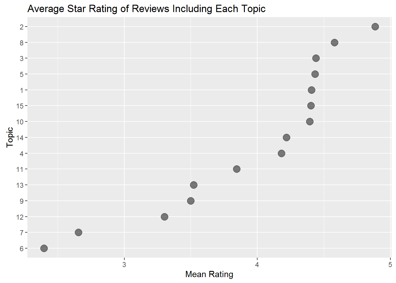
Do these star rating averages make sense in light of what the topics are?
Copyright © 2016 Karsten T. Hansen. All rights reserved.