Reshaping Data
You will on occasion have to change the organization of your data in order to accomplish a certain goal. The most common problem is the following: Your data looks like this:
| Customer | V1 | V2 | V3 | V4 | V5 |
|---|---|---|---|---|---|
| ID1 | 5 | 5 | 4 | 4 | 8 |
| ID2 | 9 | 4 | 3 | 1 | 9 |
| ID3 | 1 | 8 | 7 | 2 | 6 |
…but you want it to look like this:
| Customer | Variable | Value |
|---|---|---|
| ID1 | V1 | 5 |
| ID1 | V2 | 4 |
| ID1 | V3 | 8 |
| . | . | . |
| . | . | . |
The first version of the data is “short and wide”, while the second is “long and thin”. For example, when you import data from an Excel sheet it will often be organized with one row per customer/user and one column for each measurement. However, this is often not the ideal way to organize your data. Suppose, for example, that you are analyzing a customer satisfaction survey. Each row is a customer and you may have measured 20 to 30 different dimensions of satisfaction (e.g., ordering process, product, packaging, etc.). Now you want to summarize mean satisfaction for each dimension and different customer segments. The most elegant and efficient way of doing this is first to make the data long and thin and then do a group-by statement. Let’s look at some examples. You can download all code and data for this lesson here.
Mini-Example: States
library(tidyverse)
states <- read_rds('data/states.rds')
states
## state Population Income Life.Exp Murder HS.Grad Frost
## 1 California 21198 5114 71.71 10.3 62.6 20
## 2 Illinois 11197 5107 70.14 10.3 52.6 127
## 3 Rhode Island 931 4558 71.90 2.4 46.4 127This data is not tidy: We want each row to be a (state,measurement) combination. To make it tidy we use the gather function:
states.t <- states %>%
  gather(variable, value, Population:Frost)
This will take all the columns from Population to Frost and stack them into one column called “variable” and all the values into another column called “value”. The result is
states.t## state variable value
## 1 California Population 21198.00
## 2 Illinois Population 11197.00
## 3 Rhode Island Population 931.00
## 4 California Income 5114.00
## 5 Illinois Income 5107.00
## 6 Rhode Island Income 4558.00
## 7 California Life.Exp 71.71
## 8 Illinois Life.Exp 70.14
## 9 Rhode Island Life.Exp 71.90
## 10 California Murder 10.30
## 11 Illinois Murder 10.30
## 12 Rhode Island Murder 2.40
## 13 California HS.Grad 62.60
## 14 Illinois HS.Grad 52.60
## 15 Rhode Island HS.Grad 46.40
## 16 California Frost 20.00
## 17 Illinois Frost 127.00
## 18 Rhode Island Frost 127.00We can now easily summarize measures by state:
states.stats <- states.t %>%
  group_by(variable) %>%
  summarise(mean = mean(value))
states.stats
## # A tibble: 6 × 2
## variable mean
## <chr> <dbl>
## 1 Frost 91.333333
## 2 HS.Grad 53.866667
## 3 Income 4926.333333
## 4 Life.Exp 71.250000
## 5 Murder 7.666667
## 6 Population 11108.666667If you don’t need intermediate result later you could just use
states.stats <- states %>%
  gather(variable, value, Population:Frost) %>%
  group_by(variable) %>%
  summarise(mean = mean(value))
Example: Music Preferences
 This data contain measures of music attitudes for 48,645 users (This data is a subset of the EMI One-Million Interview dataset). For each user there is a small set of demographic information plus answers to music attitudinal questions. Attiudes are scored on a scale of 1 to 100 with higher numbers indicating stronger agreement with the corresponding attitude. First load the data:
load('data/music.rda') There are two data frames in the file: users and questions. The users data frame contains the actual survey data, while questions contains labels for the survey questions. Let’s take a look at the first three rows of the survey data:
users[1:3,]## RESPID GENDER AGE WORKING REGION
## 1 36927 Female 60 Other South
## 2 3566 Female 36 Full-time housewife / househusband South
## 3 20054 Female 52 Employed 30+ hours a week Midlands
## MUSIC
## 1 Music is important to me but not necessarily more important than other hobbies or interests
## 2 Music is important to me but not necessarily more important than other hobbies or interests
## 3 I like music but it does not feature heavily in my life
## LIST_OWN LIST_BACK Q1 Q2 Q3 Q4 Q5 Q6 Q7 Q8 Q9 Q10 Q11 Q12 Q13
## 1 1 hour 49 50 49 50 32 33 32 0 74 50 50 71 52
## 2 1 hour 1 hour 55 55 62 9 9 9 10 11 55 12 65 65 80
## 3 1 hour Less than an hour 11 50 9 8 45 10 30 29 8 50 94 51 74
## Q14 Q15 Q16 Q17 Q18 Q19
## 1 71 9 7 72 49 26
## 2 79 51 31 68 54 33
## 3 66 27 46 73 8 31This data is clearly short and wide: there is one row per respondent. We want to make it long and thin instead, with each row corresponding to one (user,measurement) combination. The 19 attitudinal questions are labelled Q1-Q19. You can see their labels in the questions data frame.
To reshape data we can use the tidyr package. The main command we will use is gather. Try out the following:
users.tidy <- users %>%
  gather(attitude,value,Q1:Q19)
What did this do? If you check the dimensions of the new data frame users.tidy, you will see that it has 924,255 rows. This is exactly 19 times the number of rows of the users data frame. This happened because the gather command stacked all the 19 attitudes into one column (that we decided to call attitude).
It is now very easy to summarize attitudes by numerical summaries or visualizations. For example, what is the average attitude score for each of the 19 attitudes? Easy:
users.tidy %>%
  group_by(attitude) %>%
  summarize(mean=mean(value,na.rm=TRUE))
## # A tibble: 19 × 2
## attitude mean
## <chr> <dbl>
## 1 Q1 49.11357
## 2 Q10 55.01103
## 3 Q11 58.63643
## 4 Q12 53.66590
## 5 Q13 46.96266
## 6 Q14 53.44644
## 7 Q15 39.66456
## 8 Q16 35.57926
## 9 Q17 53.82629
## 10 Q18 42.23245
## 11 Q19 41.36263
## 12 Q2 54.62442
## 13 Q3 51.28445
## 14 Q4 37.30913
## 15 Q5 34.58543
## 16 Q6 39.33361
## 17 Q7 33.84533
## 18 Q8 29.16174
## 19 Q9 47.83174Do these averages differ for men and women? Let’s check by doing a visualization:
users.tidy %>%
  group_by(GENDER,attitude) %>%
  summarize(mean=mean(value,na.rm=TRUE)) %>%
  ggplot(aes(x=attitude,fill=GENDER,y=mean)) + geom_bar(stat='identity',position='dodge')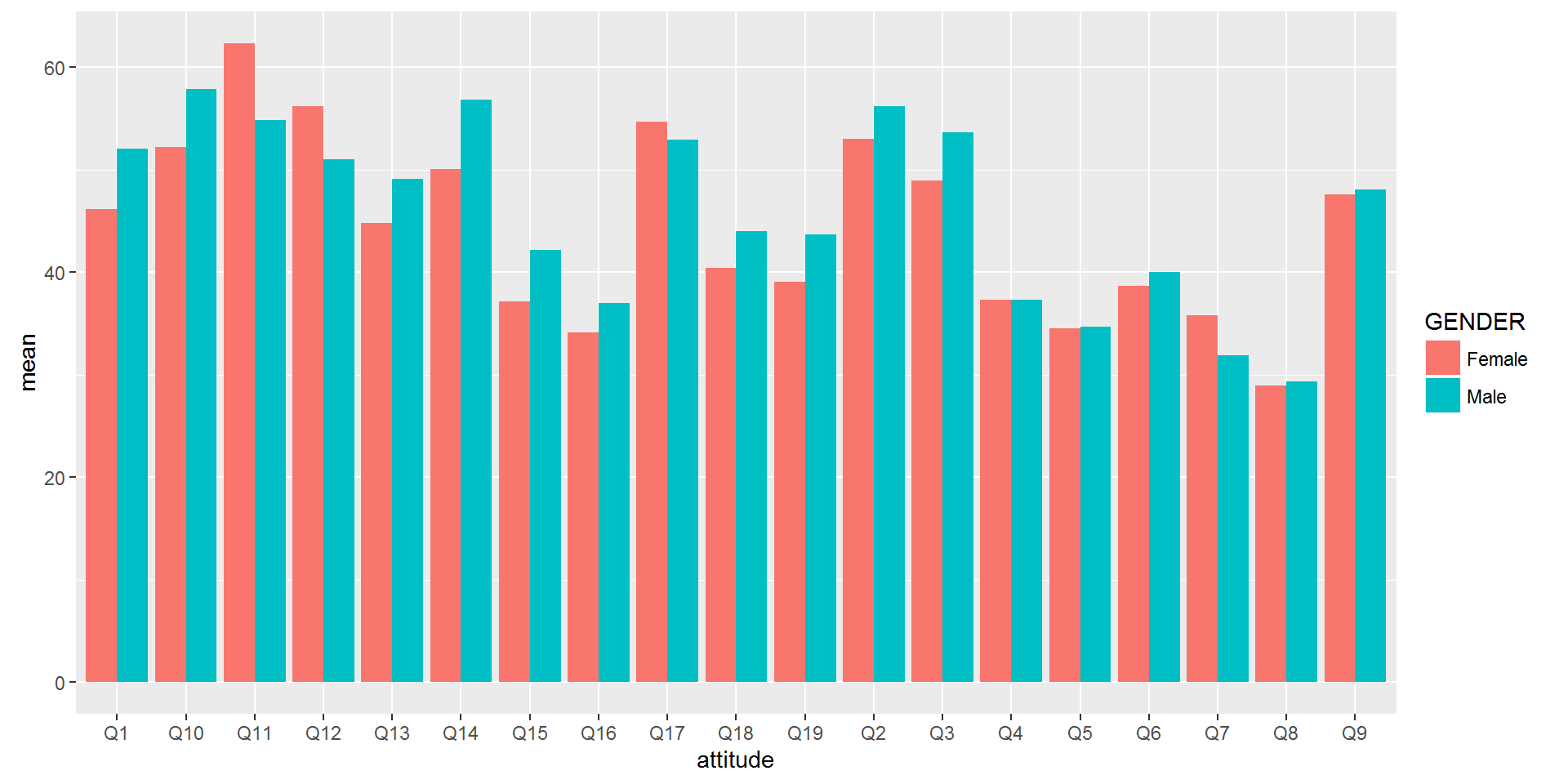
Let’s plot the average scores for each gender for the attitudes where the gender difference is the biggest, using the correct attitude labels:
users.tidy %>%
  group_by(GENDER,attitude) %>%
  summarize(mean=mean(value,na.rm=TRUE)) %>%
  filter(attitude %in% c('Q1','Q11','Q14')) %>%
  left_join(questions,by=c('attitude'='variable')) %>%
  ggplot(aes(x=label,fill=GENDER,y=mean)) + geom_bar(stat='identity',position='dodge') + coord_flip()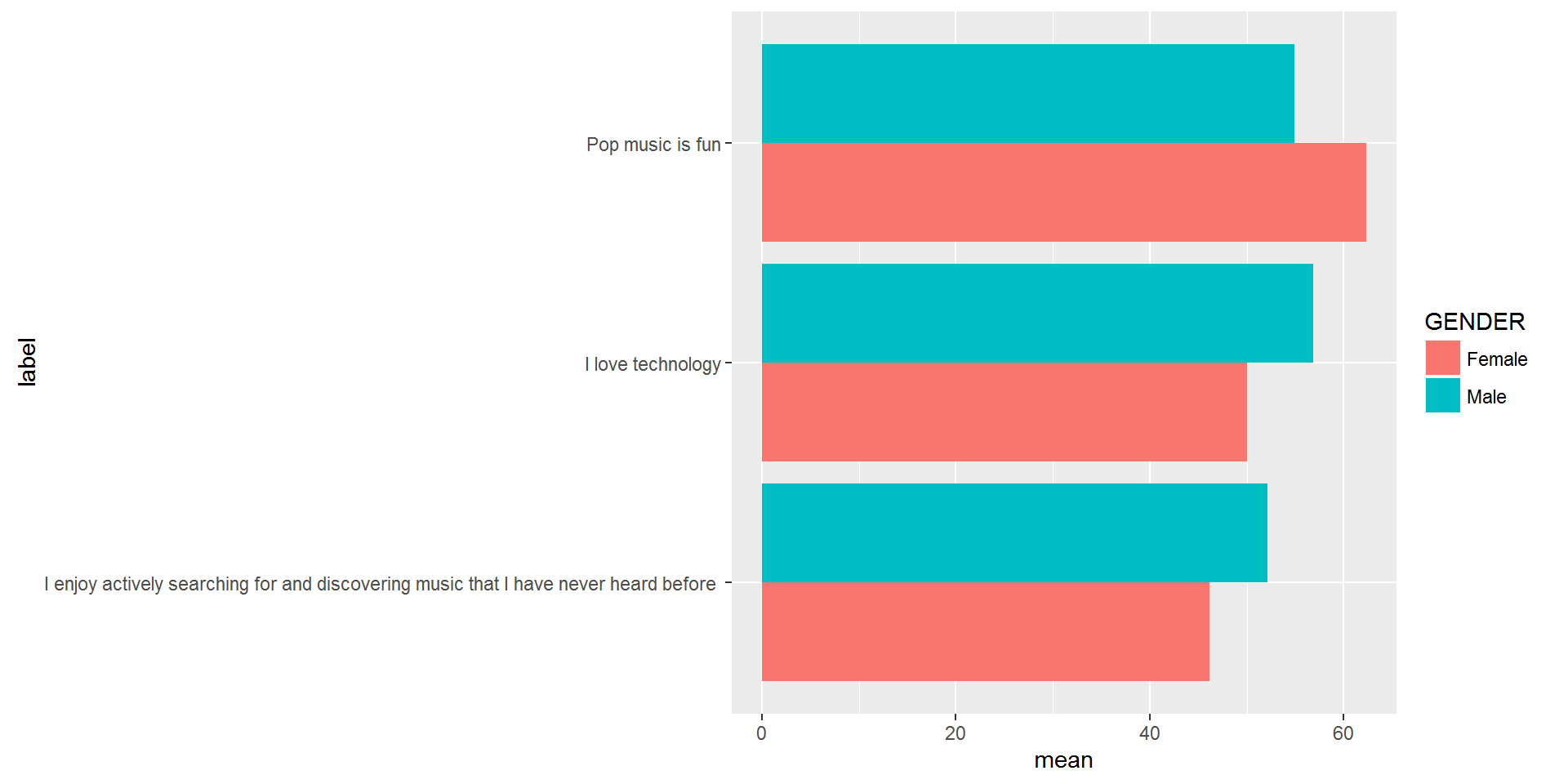
Exercise
The variable MUSIC capures how important music is to the respondent overall. Summarize the average attitude Q1-Q19 for each level of MUSIC. Do you see any differences? Do the differences make sense?
Copyright © 2016 Karsten T. Hansen. All rights reserved.