Summarizing a Corpus
Text data is messy and to make sense of it you often have to clean it a bit first. For example, do you want “Tuesday” and “Tuesdays” to count as separate words or the same word? Most of the time we would want to count this as the same word. Similarly with “run” and “running”. Furthermore, we often are not interested in including punctuation in the analysis - we just want to treat the text as a “bag of words”. There are libraries in R that will help you do this.
All code and data for this and the other two modules on text mining can be fond in this zip file.
In the following let’s look at Yelp reviews of Las Vegas hotels:
load('vegas_hotels.rda')This data contains customer reviews of 18 hotels in Las Vegas. We can use the ggmap library to plot the hotel locations:
library(ggmap)
ggmap(get_map("The Strip, Las Vegas, Nevada",zoom=15,color = "bw")) +
    geom_text(data=business,
              aes(x=longitude,y=latitude,label=name),
size=3,color='red') 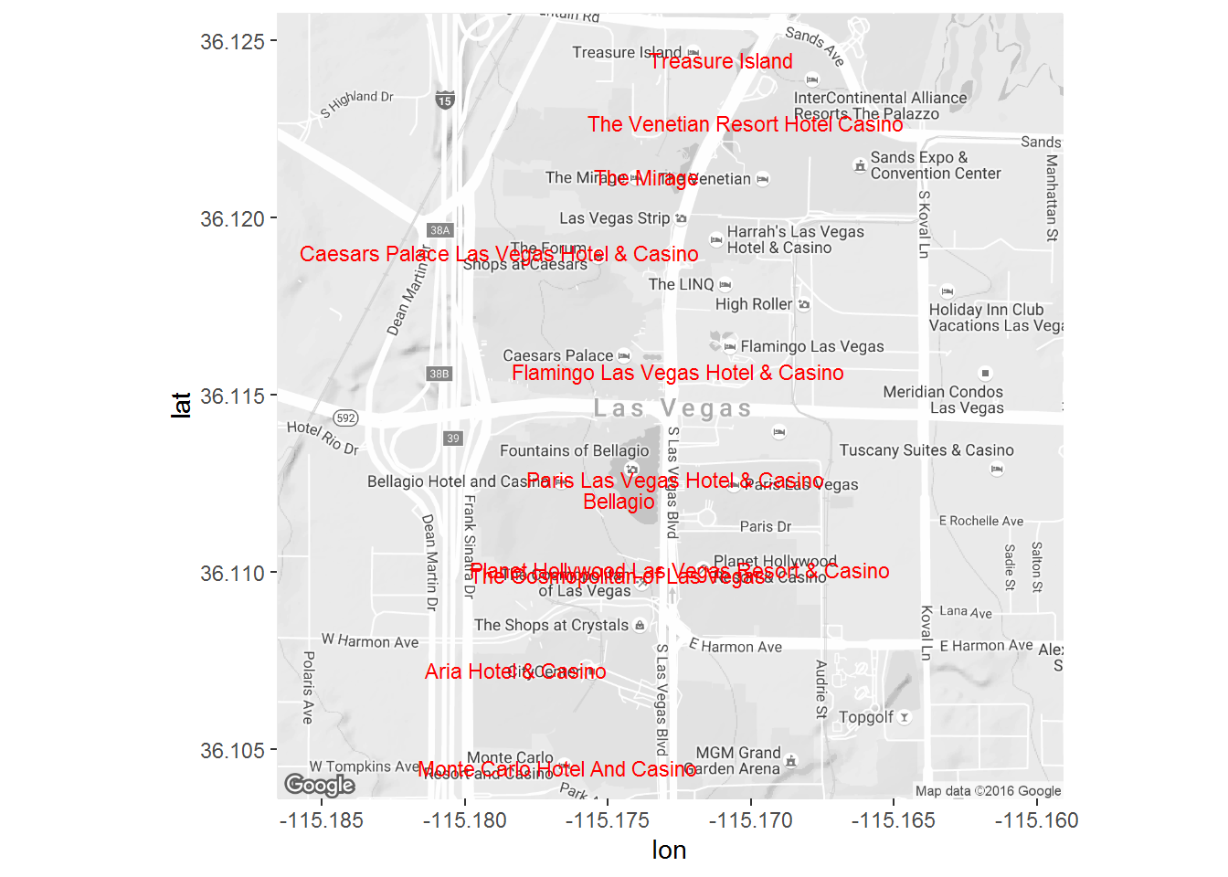
In addition to text, each review also contain a star rating from 1 to 5. Let’s see how the 18 hotels fare on average in terms of star ratings:
library(tidyverse)
library(scales)

reviews %>%
  left_join(select(business,business_id,name),
             by='business_id') %>%
  group_by(name) %>%
  summarize(n = n(),
            mean.star = mean(as.numeric(stars))) %>%
  arrange(desc(mean.star)) %>%
  ggplot() +
  geom_point(aes(x=reorder(name,mean.star),y=mean.star,size=n))+
  coord_flip() +
  ylab('Mean Star Rating (1-5)') +
  xlab('Hotel')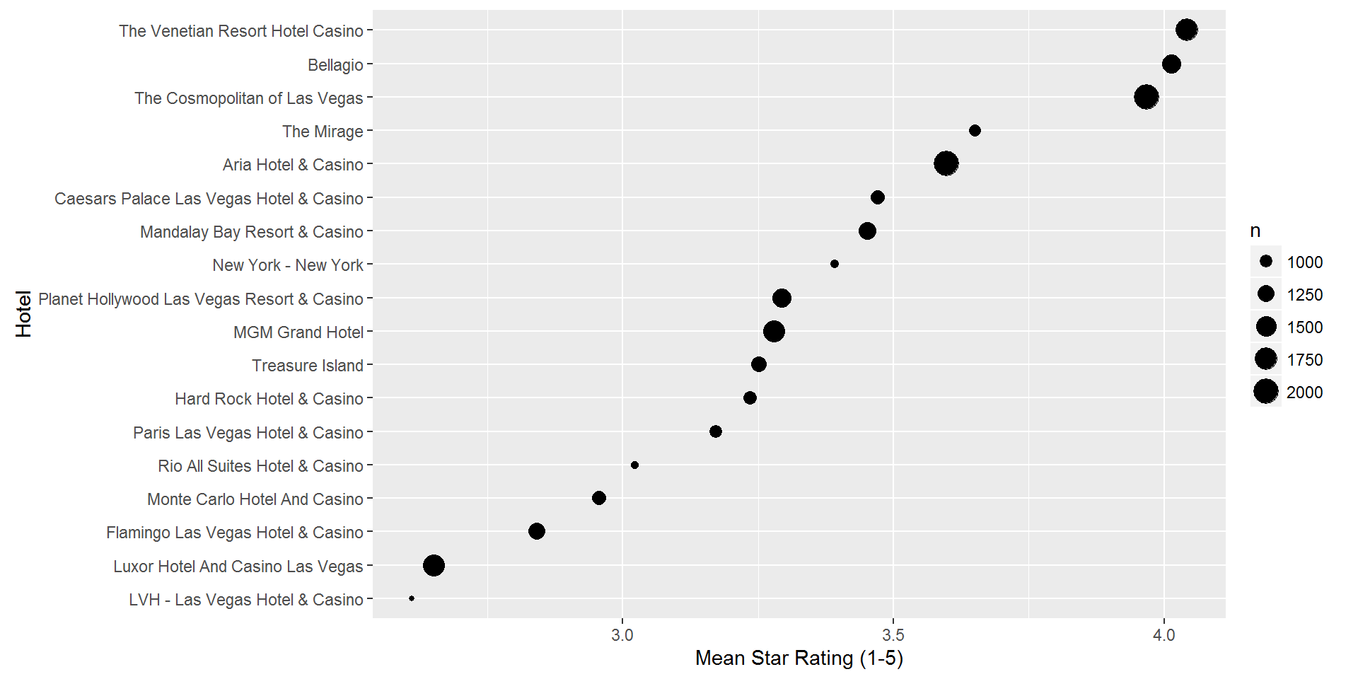
So The Venetian, Bellagio and The Cosmopolitan are clearly the highest rated hotels, while Luxor and LVH are the lowest rated. Ok, but what is behind these ratings? What are customers actually saying about these hotels? This is what we can hope to find through a text analysis.
Constructing a Document Term Matrix
In the follwing we will make use of three libraries for text mining:
## install packages
install.packages(c("tm","wordcloud","tidytext"))  ## only run once
library(tm)
library(tidytext)
library(wordcloud)
The foundation of a text analysis is a document term matrix. This is an array where each row corresponds to a document and each column corresponds to a word. The entries of the array are simply counts of how many times a certain word occurs in a certain document. Let’s look at a simple example:
example <- data.frame(document=c(1:4),
                the.text=c("I have a brown dog. My dog loves walks.",
                       "My dog likes food.",
                       "I like food.",
                       "Some dogs are black."))
This data contains four documents. The first document contains 8 unique words (or “terms”). The word “brown” occurs once while “dog” occurs twice.
library(tm)

text.c <- VCorpus(DataframeSource(select(example,the.text)))
DTM <- DocumentTermMatrix(text.c,
                          control=list(removePunctuation=TRUE,
                                       wordLengths=c(1, Inf)))
inspect(DTM)
## <<DocumentTermMatrix (documents: 4, terms: 15)>>
## Non-/sparse entries: 19/41
## Sparsity : 68%
## Maximal term length: 5
## Weighting : term frequency (tf)
##
## Terms
## Docs a are black brown dog dogs food have i like likes loves my some walks
## 1 1 0 0 1 2 0 0 1 1 0 0 1 1 0 1
## 2 0 0 0 0 1 0 1 0 0 0 1 0 1 0 0
## 3 0 0 0 0 0 0 1 0 1 1 0 0 0 0 0
## 4 0 1 1 0 0 1 0 0 0 0 0 0 0 1 0The first statement creates a corpus from the data frame example using the the.text variable. Then we create a document term matrix using this corpus. The control statement tells R to keep terms of any length (without this short words will be dropped) and to remove punctuation before creating the DTM.
In addition to removing punctuation (and lower-casing terms which is done by default) there are two other standard “cleaning” operations which are usually done. The first is to removed stopwords from the corpus. Stopwords are common words in a language that (usually) doesn’t carry any important significance in the analysis. For example, we could replace the first document in the example with “brown dog loves walks” and still be able to infer that the person writing this document talks about a brown dog. Of course, some information is lost in this process but for many applications this is not really an issue. The second standard operation is stemming. This creates root words, e.g., turns dogs into dog and loves into love:
text.c <- VCorpus(DataframeSource(select(example,the.text)))
DTM <- DocumentTermMatrix(text.c,
                          control=list(removePunctuation=TRUE,
                                       wordLengths=c(1, Inf),
                                       stopwords=TRUE,
                                       stemming=TRUE
                                       ))
inspect(DTM)
## <<DocumentTermMatrix (documents: 4, terms: 7)>>
## Non-/sparse entries: 11/17
## Sparsity : 61%
## Maximal term length: 5
## Weighting : term frequency (tf)
##
## Terms
## Docs black brown dog food like love walk
## 1 0 1 2 0 0 1 1
## 2 0 0 1 1 1 0 0
## 3 0 0 0 1 1 0 0
## 4 1 0 1 0 0 0 0If you are not sure about a stemmed term’s origin you can look it up in the stem vocabulary:
stem.voc <- read_rds('data/stem_voc.rds')Here are all the origin words for “love”:
filter(stem.voc,Stem=="love")## # A tibble: 5 × 2
## Original Stem
## <chr> <chr>
## 1 love love
## 2 loved love
## 3 lovely love
## 4 loves love
## 5 loving loveNow let’s return to the hotel reviews. Let’s try to summarize the reviews for the Aria hotel:
aria.id <-  filter(business,
        name=='Aria Hotel & Casino')$business_id
aria.reviews <- filter(reviews,
         business_id==aria.id)
Next, we construct the DTM by using the operations described above (and we also remove numbers from the reviews). We inspect the first 10 documents and 10 terms:
text.c <- VCorpus(DataframeSource(select(aria.reviews,text)))


meta.data <- aria.reviews %>%
  select(stars,votes.funny,votes.useful,votes.cool,date) %>%
  rownames_to_column(var="document")


DTM.aria <- DocumentTermMatrix(text.c,
                          control=list(removePunctuation=TRUE,
                                       wordLengths=c(3, Inf),
                                       stopwords=TRUE,
                                       stemming=TRUE,
                                       removeNumbers=TRUE
                                       ))
inspect(DTM.aria[1:10, 1:10])
## <<DocumentTermMatrix (documents: 10, terms: 10)>>
## Non-/sparse entries: 0/100
## Sparsity : 100%
## Maximal term length: 9
## Weighting : term frequency (tf)
##
## Terms
## Docs aaa aaah aaauugghh aaay aah aback abandon abbrevi abc aberr
## 1 0 0 0 0 0 0 0 0 0 0
## 2 0 0 0 0 0 0 0 0 0 0
## 3 0 0 0 0 0 0 0 0 0 0
## 4 0 0 0 0 0 0 0 0 0 0
## 5 0 0 0 0 0 0 0 0 0 0
## 6 0 0 0 0 0 0 0 0 0 0
## 7 0 0 0 0 0 0 0 0 0 0
## 8 0 0 0 0 0 0 0 0 0 0
## 9 0 0 0 0 0 0 0 0 0 0
## 10 0 0 0 0 0 0 0 0 0 0Ok - here we can already see a problem: Users are writing all kinds of weird stuff in their reviews! You know - stuff like “aaauugghh”. Terms like these are likely to occur in only a very few documents, which means that we should probably just get rid of them. To see how many unique terms actually are in the DTM we can just print it:
print(DTM.aria)## <<DocumentTermMatrix (documents: 2011, terms: 10197)>>
## Non-/sparse entries: 158219/20347948
## Sparsity : 99%
## Maximal term length: 117
## Weighting : term frequency (tf)There are a total of 10,197 terms. That’s a lot and many of them are meaningless and sparse, i.e., they only occur in a few documents. The following command will remove terms that doesn’t occur in 99.5% of documents
DTM.aria.sp <- removeSparseTerms(DTM.aria,0.995)
inspect(DTM.aria.sp[1:10, 1:10])
## <<DocumentTermMatrix (documents: 10, terms: 10)>>
## Non-/sparse entries: 2/98
## Sparsity : 98%
## Maximal term length: 10
## Weighting : term frequency (tf)
##
## Terms
## Docs abl absolut accept access accident accommod account acknowledg across
## 1 0 0 0 0 0 0 0 0 0
## 2 0 0 0 0 0 0 0 0 0
## 3 0 0 0 0 0 0 0 0 0
## 4 0 0 0 0 0 0 0 0 0
## 5 0 0 0 0 0 0 0 0 0
## 6 0 0 0 0 0 0 0 0 0
## 7 0 0 0 0 0 0 0 0 0
## 8 0 0 0 0 0 1 0 0 0
## 9 0 0 0 0 0 0 0 0 0
## 10 0 0 0 0 0 0 0 0 0
## Terms
## Docs act
## 1 0
## 2 0
## 3 0
## 4 0
## 5 1
## 6 0
## 7 0
## 8 0
## 9 0
## 10 0This looks much better. We now have a lot fewer terms in the DTM:
print(DTM.aria.sp)## <<DocumentTermMatrix (documents: 2011, terms: 1788)>>
## Non-/sparse entries: 140761/3454907
## Sparsity : 96%
## Maximal term length: 13
## Weighting : term frequency (tf)So by removing all the sparse terms we want from 10,197 to 1,788 terms.
Summarizing a Document Term Matrix
Now that we have creating our document term matrix, we can start summarizing the corpus. What are the most frequent terms? Easy:
library(forcats)

aria.tidy <- tidy(DTM.aria.sp)

term.count <- aria.tidy %>%
  group_by(term) %>%
  summarize(n.total=sum(count)) %>%
  arrange(desc(n.total))


term.count %>%
  slice(1:30) %>%
  ggplot(aes(x=fct_reorder(term,n.total),y=n.total)) + geom_bar(stat='identity') +
  coord_flip() + xlab('Counts') + ylab('')+ggtitle('Most Frequent Terms')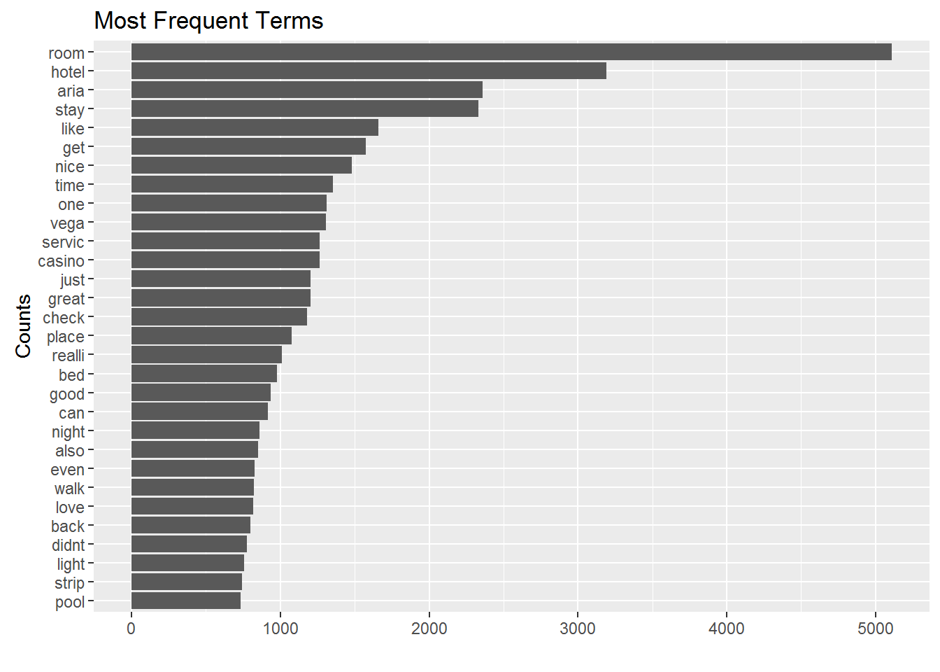
A popular visualization tools of term counts is a word cloud. This is simply an alternative visual representation of the counts. We can easily make one:
library(wordcloud)

term.count.pop <- term.count %>%
  slice(5:100)

wordcloud(term.count.pop$term, term.count.pop$n.total, scale=c(5,.5))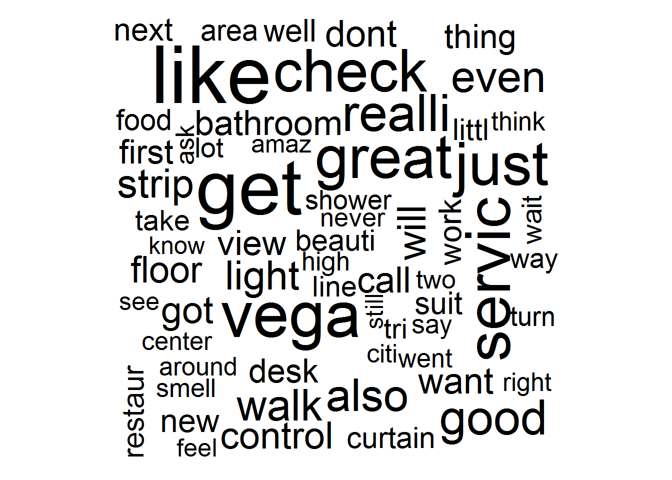
Ok, now let’s look at associations between terms. When people talk about “room”, what other terms are used?
room <- data.frame(findAssocs(DTM.aria.sp, "room", 0.35)) # find terms correlated with "room"

room %>%
  rownames_to_column() %>%
  ggplot(aes(x=reorder(rowname,room),y=room)) + geom_point(size=4) +
  coord_flip() + ylab('Correlation') + xlab('Term') +
  ggtitle('Terms correlated with Room')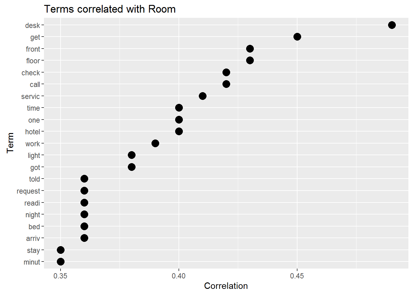
This seems to be terms related to the check-in process. This is something that can be explored in more detail using topic models.
How about “bathroom”?
bathroom <- data.frame(findAssocs(DTM.aria.sp, "bathroom", 0.2))

bathroom %>%
  rownames_to_column() %>%
  ggplot(aes(x=reorder(rowname,bathroom),y=bathroom)) + geom_point(size=4) +
  coord_flip() + ylab('Correlation') + xlab('Term') +
  ggtitle('Terms correlated with Bathroom')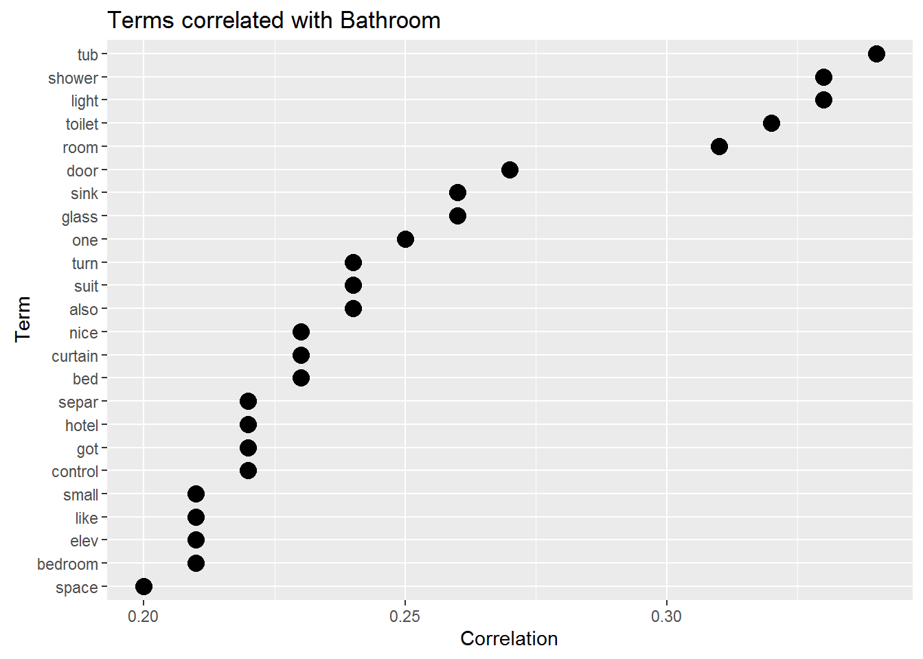
When talking about the bathroom users are most likely to mention “tub”“,”shower“,”light“,”toilet" and “room”.
Exercise 1
In the analysis above we pooled all users into one segment. This may be quite misleading for a heterogenous set of users. For example, we might suspect that satisfied and non-satisified users talk about different things - or talk differently about the same things.
- To look into this consider separate analyses for satisfied and non-satisfied visitors (with satisfied visitors defined as having 5 star rated reviews and non-satisfied visitors having 1 or 2 star reviews).
- Are the most frequently used words the same for the two segments?
- Find terms correlated with “desk” and “valet” for each segment. Is it the same words? Do the correlated terms make sense?
Note that this exercise requires that you join the review meta-data with the review text. You can do this easily like this
aria.tidy.meta <- aria.tidy %>%
  inner_join(meta.data,by="document")
You now have the star ratings associated with each document. For finding word associations it is useful to return to the document-term matrix structure. You can go from the tidy version back to the DTM version by using
dtm <- aria.tidy %>%
  cast_dtm(document, term, count)
If you combine the two you can then create DTMs for different segments. For example, the DTM for 5 star visitors can be found as
dtm5 <- aria.tidy %>%
  inner_join(meta.data,by="document") %>%
  filter(stars==5) %>%
  cast_dtm(document, term, count)
Exercise 2
Redo the analysis for different hotels - do you get the same results?
Aria v2.0
If you want to try out a much bigger database of Aria reviews, you can use the data in the file AriaReviewsTrip.rds. This contains 10,905 reviews of the Aria hotel scraped from Tripadvisor.
aria <- read_rds('data/AriaReviewsTrip.rds')

meta.data <- aria %>%
  select(reviewRating,date,year.month.group) %>%
  rownames_to_column(var="document")
With this sample size you can do more in-depth analyses. For example, how do word frequencies change over time? In the following we focus on the terms “buffet”,“pool” and “staff”. We calculate the relative frequency of these three terms for each month (relative to the total number of terms used that month).
text.c <- VCorpus(DataframeSource(select(aria,reviewText)))


DTM.aria <- DocumentTermMatrix(text.c,
                               control=list(removePunctuation=TRUE,
                                            wordLengths=c(3, Inf),
                                            stopwords=TRUE,
                                            stemming=TRUE,
                                            removeNumbers=TRUE
                               ))


DTM.aria.sp <- removeSparseTerms(DTM.aria,0.995)

aria.tidy <- tidy(DTM.aria.sp) %>%
  inner_join(meta.data,by="document")

total.terms.time <- aria.tidy %>%
  group_by(year.month.group) %>%
  summarize(n.total=sum(count))

## for the legend
a <- 1:nrow(total.terms.time)
b <- a[seq(1, length(a), 3)]

aria.tidy %>%
  filter(term %in% c("pool","staff","buffet")) %>%
  group_by(term,year.month.group) %>%
  summarize(n = sum(count)) %>%
  left_join(total.terms.time, by='year.month.group') %>%
  ggplot(aes(x=year.month.group,y=n/n.total,color=term,group=term)) +
  geom_line() +
  facet_wrap(~term)+
  theme(axis.text.x = element_text(angle = 90, hjust = 1))+
  scale_x_discrete(breaks=as.character(total.terms.time$year.month.group[b]))+
  scale_y_continuous(labels=percent)+xlab('Year/Month')+
  ylab('Word Frequency relative to Month Total')+ggtitle('Dynamics of Word Frequency for Aria Hotel')
We see three different patterns for the relative frequencies: “buffet” is used in a fairly stable manner over this time period, while “pool” displays clear seasonality, rising in popularity in the summer months. Finally, we see an upward trend in the use of “staff”.
Competitive Analysis
Here is an example of a market-wide competitive analysis using text: Compare the relative word frequency within a resort across different resorts:
text.c <- VCorpus(DataframeSource(select(reviews,text)))

meta.data <- reviews %>%
  select(business_id,stars,votes.funny,votes.useful,votes.cool,date) %>%
  rownames_to_column(var="document")

DTM.all <- DocumentTermMatrix(text.c,
                               control=list(removePunctuation=TRUE,
                                            wordLengths=c(3, Inf),
                                            stopwords=TRUE,
                                            stemming=TRUE,
                                            removeNumbers=TRUE
                               ))

all.tidy <- tidy(removeSparseTerms(DTM.all,0.995))

total.term.count.hotel <- all.tidy %>%
  inner_join(meta.data,by='document') %>%
  group_by(business_id) %>%
  summarize(n.total=sum(count))

term.count.hotel.rel <- all.tidy %>%
  inner_join(meta.data,by='document') %>%
  group_by(business_id,term) %>%
  summarize(n=sum(count)) %>%
  inner_join(total.term.count.hotel,by='business_id') %>%
  mutate(n.rel=n/n.total) %>%
  inner_join(select(business,name,business_id),by='business_id')


term.count.hotel.rel %>%
  filter(term %in% c("buffet","pool","casino","bathroom","price",
                     "shower","bad","charg","upgrad","decor")) %>%
  ggplot(aes(x=name,y=n.rel,fill=name)) + geom_bar(stat='identity') +
  facet_wrap(~term,ncol=1,scales='free_y') +
  theme(axis.text.x = element_text(angle = 45, hjust = 1))+
  theme(legend.position="none")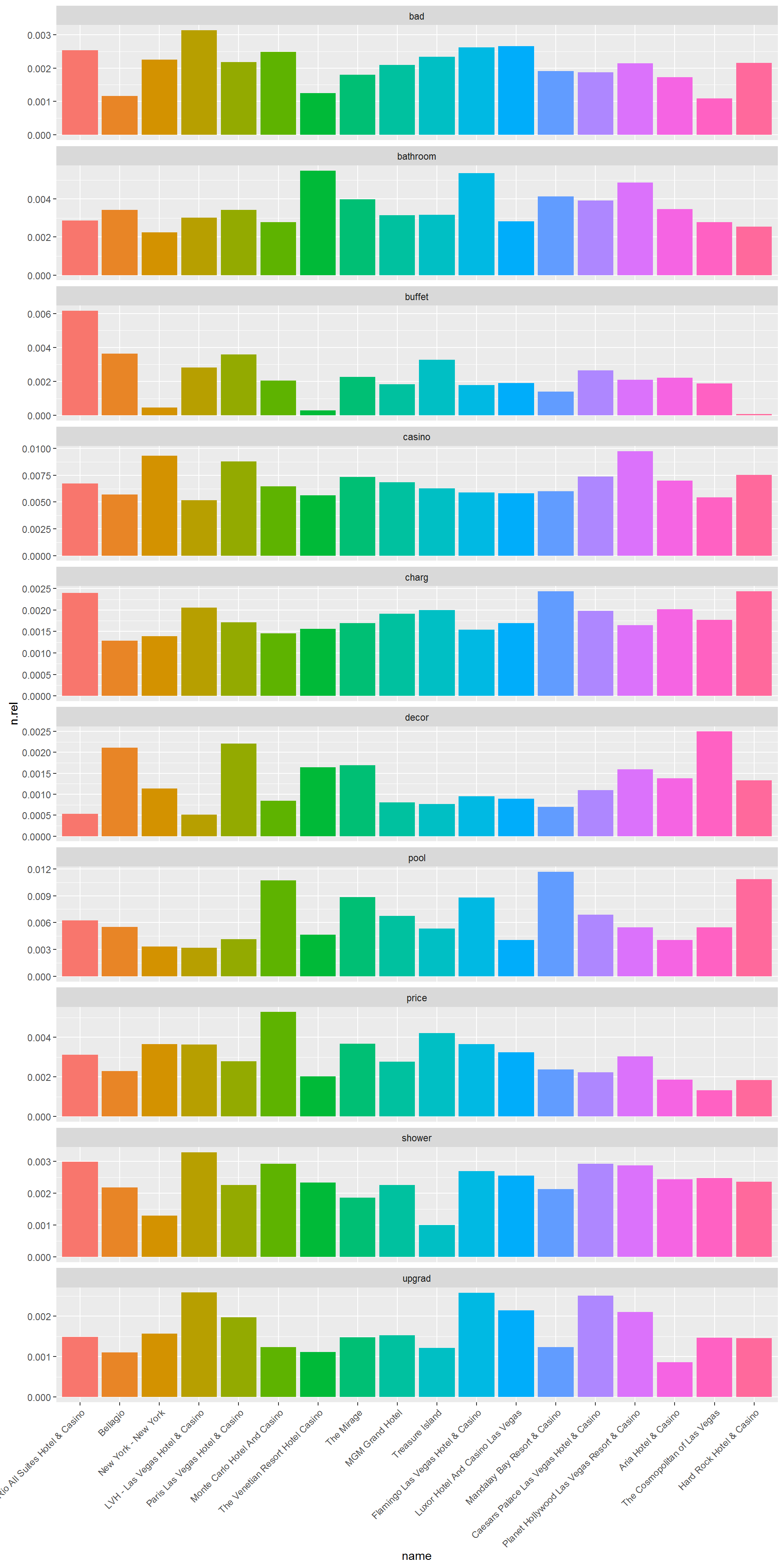
Copyright © 2016 Karsten T. Hansen. All rights reserved.