Sentiment Analysis

WWW WWW

When looking at a sentence, paragraph or entire document, it is often of interest to gauge the overall sentiment of the writer/speaker. Is it happy or sad? joyfull, fearfull or anxious? Sentiment analysis aims to accomplish this goal by assigning numerical scores to the sentiment of a set of words.

Sentiment analysis can easily be done in R using the tidytext pacakge. Consider the following three statements:

library(tidyverse)
library(tidytext)
library(tibble)
library(forcats)
library(scales)
library(tm)


sentences <- data_frame(sentence = 1:3,
                text = c("I just love this burger. It is amazing. America has the best burgers. I just love them. They are great. Someone says otherwise,  they are a loser",
                         "This burger was terrible - bad taste all around. But I did like the music in the bar.",
                         "I had a burger yesterday - it was ok. I ate all of it"))

tidy.sentences <- sentences %>%
  unnest_tokens(word,text)

This puts the text in the data frame into tidy format:

tidy.sentences

## # A tibble: 57 × 2
##    sentence    word
##       <int>   <chr>
## 1         1       i
## 2         1    just
## 3         1    love
## 4         1    this
## 5         1  burger
## 6         1      it
## 7         1      is
## 8         1 amazing
## 9         1 america
## 10        1     has
## # ... with 47 more rows

Ok - now we need to add the sentiment of each word. Note that not all words have a natural sentiment. For example, what is the sentiment of “was” or “burger”? So not all words will receive a sentiment score. The tidytext package has three sentiment lexicons built in : “afinn”, “bing” and “nrc”. The “afinn” lexicon containts negative and positive words on a scale from -5 to 5. The “bing” lexicon contains words simply coded as negative or positive sentiment. Finally, the “nrc” lexicon contains words representing the following wider range of sentiments: anger, anticipation, disgust, fear, joy, negative, positive, sadness, surprise and trust.

We can perform sentiment analysis simply by performing an inner join operation:

tidy.sentences %>%
  inner_join(get_sentiments("bing"),by="word")

## # A tibble: 9 × 3
##   sentence     word sentiment
##      <int>    <chr>     <chr>
## 1        1     love  positive
## 2        1  amazing  positive
## 3        1     best  positive
## 4        1     love  positive
## 5        1    great  positive
## 6        1    loser  negative
## 7        2 terrible  negative
## 8        2      bad  negative
## 9        2     like  positive

Only words contained in the bing lexicon shows up. We see that the first sentence contained 5 positive words, while the second contained 2 negative and 1 positive. Notice that the word “love” occurs twice in the first sentence so it makes sense to weigh it higher than “amazing” that only occurs once. We can do this by first doing a term count before joining the sentiments:

tidy.sentences %>%
  count(sentence,word) %>%
  inner_join(get_sentiments("bing"),by="word")

## Source: local data frame [8 x 4]
## Groups: sentence [?]
## 
##   sentence     word     n sentiment
##      <int>    <chr> <int>     <chr>
## 1        1  amazing     1  positive
## 2        1     best     1  positive
## 3        1    great     1  positive
## 4        1    loser     1  negative
## 5        1     love     2  positive
## 6        2      bad     1  negative
## 7        2     like     1  positive
## 8        2 terrible     1  negative

Notice that the third sentence disappeared as it consisted only of neutral words. We can now tally the total sentiment for each sentence:

tidy.sentences %>%
  count(sentence,word) %>%
  inner_join(get_sentiments("bing"),by="word") %>%
  group_by(sentence,sentiment) %>%
  summarize(total=sum(n))

## Source: local data frame [4 x 3]
## Groups: sentence [?]
## 
##   sentence sentiment total
##      <int>     <chr> <int>
## 1        1  negative     1
## 2        1  positive     5
## 3        2  negative     2
## 4        2  positive     1

Finally, we can calculate a net-sentiment by subtracting positive and negative sentiment:

tidy.sentences %>%
  count(sentence,word) %>%
  inner_join(get_sentiments("bing"),by="word") %>%
  group_by(sentence,sentiment) %>%
  summarize(total=sum(n)) %>%
  spread(sentiment,total) %>%
  mutate(net.positve=positive-negative)

## Source: local data frame [2 x 4]
## Groups: sentence [2]
## 
##   sentence negative positive net.positve
##      <int>    <int>    <int>       <int>
## 1        1        1        5           4
## 2        2        2        1          -1

Case Study: Clinton vs. Trump Convention Acceptance Speeches

To illustrate the ease with which one can do sentiment analysis in R, let’s look at all dimensions of sentiment in the democrat and republican convention acceptance speeches by Hillary Clinton and Donald Trump. The convention_speeches.rds file contains the transcript of each speech.

speech <- read_rds('data/convention_speeches.rds')

tidy.speech <- speech %>%
  unnest_tokens(word,text) 

total.terms.speaker <- tidy.speech %>%
  count(speaker)

The total number of terms in each speech is

total.terms.speaker

## # A tibble: 2 × 2
##   speaker     n
##     <chr> <int>
## 1 clinton  5427
## 2   trump  5161

Let’s break down the total number of terms into the different sentiments and plot the relative frequency of each:

sentiment.orientation <- data.frame(orientation = c(rep("Positive",5),rep("Negative",5)),
                                sentiment = c("anticipation","joy","positive","trust","surprise","anger","disgust","fear","negative","sadness"))

tidy.speech %>%
  count(speaker,word) %>%
  inner_join(get_sentiments("nrc"),by=c("word")) %>%
  group_by(speaker,sentiment) %>%
  summarize(total=sum(n)) %>%
  inner_join(total.terms.speaker) %>%
  mutate(relative.sentiment=total/n) %>%
  inner_join(sentiment.orientation) %>%
  ggplot(aes(x=sentiment,y=relative.sentiment,fill=speaker)) + geom_bar(stat='identity',position='dodge') + 
  facet_wrap(~orientation,scales='free')+
  ylab('Relative Sentiment')+
  labs(title='Sentiment of Convention Acceptance Speeches',
       subtitle='Hillary Clinton vs. Donald Trump')+
  scale_y_continuous(labels=percent)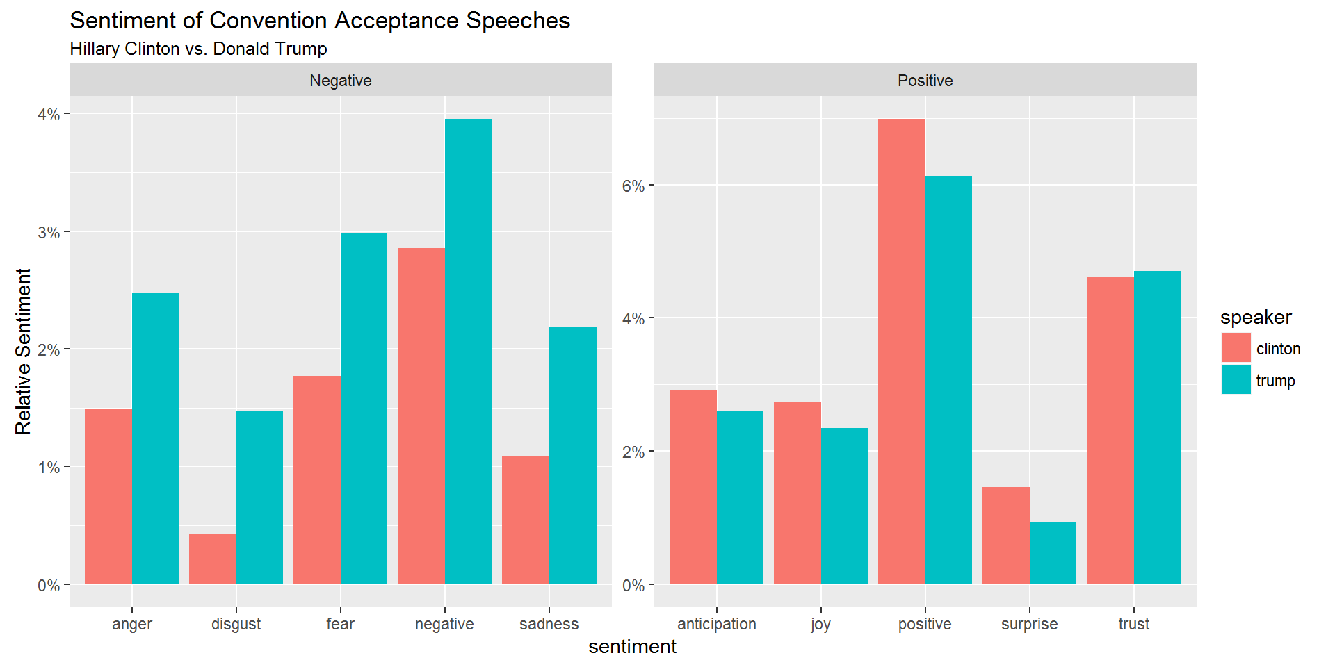

Case Study: Fear and Loathing - Sentiments in Las Vegas

Let’s return to the Las Vegas resort reviews and study how average sentiment vary across resorts. We start by loading the review data, cleaning it up and convert to tidy text:

load('data/vegas_hotels.rda')

text.c <- VCorpus(DataframeSource(select(reviews,text)))

meta.data <- reviews %>%
  select(stars,votes.funny,votes.useful,votes.cool,date,business_id) %>%
  rownames_to_column(var="document")

DTM.all <- DocumentTermMatrix(text.c,
                               control=list(removePunctuation=TRUE,
                                            wordLengths=c(3, Inf),
                                            stopwords=TRUE,
                                            removeNumbers=TRUE
                               ))


reviews.tidy <- tidy(removeSparseTerms(DTM.all,0.999))

Suppose we were interested in the negative and positive sentiment for each resort and the difference between the two, i.e., the net positive sentiment. To do this, first calculate the total number of terms used for each resort:

term.hotel <- reviews.tidy %>%
  left_join(select(meta.data,business_id,document),by='document') %>%
  group_by(business_id) %>%
  summarize(n.hotel=sum(count))

Next we join in the sentiment lexicon, summarize total sentiment for each hotel, normalize by total term count by hotel and finally join in the hotel name and visualize the result:

bing <- get_sentiments("bing") 

hotel.sentiment <- reviews.tidy %>%
  inner_join(bing,by=c("term"="word")) %>%
  left_join(select(meta.data,business_id,document),by='document') %>%
  group_by(business_id,sentiment) %>%
  summarize(total=sum(count)) %>%
  inner_join(term.hotel,by='business_id') %>%
  mutate(relative.sentiment = total/n.hotel) %>%
  inner_join(select(business,business_id,name),by='business_id')


hotel.sentiment %>%
  ggplot(aes(x=sentiment,y=relative.sentiment,fill=sentiment)) + geom_bar(stat='identity') + 
  facet_wrap(~name)+ theme(axis.text.x = element_text(angle = 45, hjust = 1))

This is a nice visualization but to see the actual net positive sentiment differences across hotels, this one is probably better:

hotel.sentiment %>%
  select(sentiment,relative.sentiment,name) %>%
  spread(sentiment,relative.sentiment) %>%
  mutate(net.pos = positive-negative) %>%
  ggplot(aes(x=fct_reorder(name,net.pos),y=net.pos)) + geom_point(size=4) + coord_flip()+
  scale_y_continuous(labels=percent)+ylab('Net Positive Sentiment')+xlab('Resort')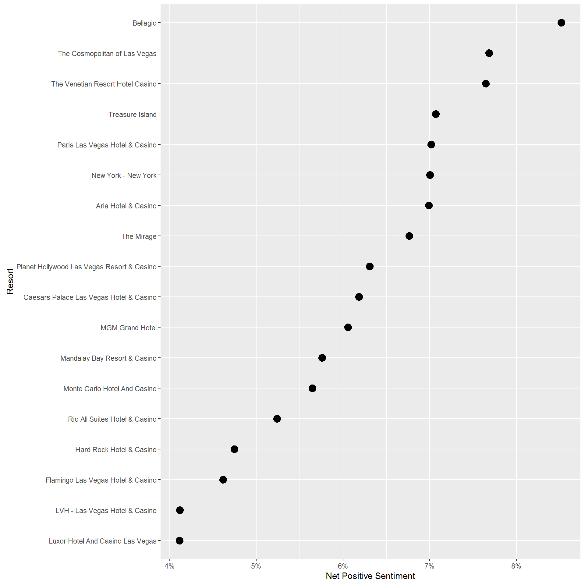

nrc <- get_sentiments("nrc")

hotel.sentiment <- reviews.tidy %>%
  inner_join(nrc,by=c("term"="word")) %>%
  left_join(select(meta.data,business_id,document),by='document') %>%
  group_by(business_id,sentiment) %>%
  summarize(total=sum(count)) %>%
  inner_join(term.hotel,by='business_id') %>%
  mutate(relative.sentiment = total/n.hotel) %>%
  inner_join(select(business,business_id,name),by='business_id')

hotel.sentiment %>%
  filter(!sentiment %in% c("disgust","fear")) %>%
  ggplot(aes(x=sentiment,y=relative.sentiment,fill=sentiment)) + geom_bar(stat='identity') + 
  facet_wrap(~name,ncol=3)+ theme(axis.text.x = element_text(angle = 45, hjust = 1)) + 
  theme(legend.position="none")

Exercise

If sentiment analysis is worth anything, then positive vs. negative sentiment of a review should be able to predict the star rating. In this exercise you will investigate if this is true.

Using the reviews.tidy and meta.data from above follow the following steps:

Join the sentiments from the “afinn” lexicon with the reviews.tidy data frame.
Look at the resulting data frame and make sure you understand the result
Then for each document calculate the total sentiment score (remember that in the afinn lexicon words are given a score from -5 to 5 where higher is more positive)
Join the meta.data to the result in 3.

Using your resulting data frame in 4., what can you say about the relationship between sentiments and star rating?