Relational Databases in R

In many situations your data will be stored in separate files with dimensions defined by the nature of the objects that the data represents. For example, a large transactional database might contain four individual files (or “tables”): (1) a transaction file (2) a product file (3) a customer file and (4) a store file. Each of these will contain different information that can be linked to each other. This is also called a relational database since the objects stored in it can be linked or related to each other.
You can download data and code for this module as an Rstudio project here. You should unzip this file somewhere on you computer’s hard drive and then open the file Relational data.Rproj in Rstudio.
Here is a simple example of a relational database: Suppose you have data on the results of two running races. Each set of race results form a table. A third table contains a list of runners, while a fourth contains the list of races. These four tables define a relational database:
load('data/run_race_database.rda')

Race1Results

Race2Results

Runners

Races
## RaceId RunnerId RaceTime
## 1 1 1 100
## 2 1 2 120
## 3 1 3 90
## 4 1 4 140## RaceId RunnerId RaceTime
## 1 2 2 115
## 2 2 4 145
## 3 2 5 105
## 4 2 6 95## RunnerId Name Gender Age
## 1 1 Peter M 35-39
## 2 2 Jenny F 30-34
## 3 3 Heather F 25-29
## 4 4 John M 30-34
## 5 5 Max M 35-39
## 6 6 Julie F 40-44## RaceId RaceName
## 1 1 La Jolla Half Marathon
## 2 2 Silver Strand Half MarathonThere are multiple relationships across tables in this database. For example, we can link the same runners across races or we can link runner characteristics to race results or race name to results. All of these operations require us to join tables which is the standard operation done on relational databases. Once the join operation is done, we can continue with other summary operations, visualizations or other more advanced analytics tools.
There are different join operations available depending on what your objective is. First, suppose you are interested in comparing the same runner’s performance across different races. In this case we need to extract results for runners who show up in both of the two race results tables. You can think of this as the intersection between the two tables. This is done by using the inner_join function:
library(tidyverse)
RunnersRace12 <- inner_join(Race1Results, Race2Results, by = 'RunnerId')
RunnersRace12
## RaceId.x RunnerId RaceTime.x RaceId.y RaceTime.y
## 1 1 2 120 2 115
## 2 1 4 140 2 145Notice that R renamed the race specific variables by adding an “x” and “y”. This is because the RaceId and RaceTime variable has the same name in Race1Result and Race2Result and we obviously need to distinguish between them. The “by” option informs R on which variable the join operation is to be performed. There may situations where you want the racers who ran both races (the intersection) but you only want the results from the first race. You can do this with a semi_join :
RunnersRace12 <- semi_join(Race1Results, Race2Results, by = 'RunnerId')
RunnersRace12
## RaceId RunnerId RaceTime
## 1 1 2 120
## 2 1 4 140Suppose instead that you were interested in a “master” race file that had information on all races for all runners. You can think of this as the union of the race 1 and race 2 table. You can do this operation by using full_join:
RunnersRace12All <- full_join(Race1Results, Race2Results, by = 'RunnerId')
RunnersRace12All
## RaceId.x RunnerId RaceTime.x RaceId.y RaceTime.y
## 1 1 1 100 NA NA
## 2 1 2 120 2 115
## 3 1 3 90 NA NA
## 4 1 4 140 2 145
## 5 NA 5 NA 2 105
## 6 NA 6 NA 2 95Notice that we now have a bunch of NAs (=“Not Available” - this is how R represents missing data) in the merged result. That is because the result - being the union of the two race tables - has one row with all race results for each runner and several runners only ran in one race.
Suppose instead you wanted to extract the race data for all races that runners who ran race 1 has ever run. This can be accomplished by a left_join operation:
RunnersRace1All <- left_join(Race1Results, Race2Results, by = 'RunnerId')
RunnersRace1All
## RaceId.x RunnerId RaceTime.x RaceId.y RaceTime.y
## 1 1 1 100 NA NA
## 2 1 2 120 2 115
## 3 1 3 90 NA NA
## 4 1 4 140 2 145Finally, you may sometimes be interested in extracting the records that do not overlap between two tables rather than the ones that do. For example, suppose you were interested in the runners who ran in race 1 but not in race 2. You can think of this as the complement of the inner join operation above when compared to the original race 1 table. This can be generated by using an anti_join operation:
Race1Only <- anti_join(Race1Results,Race2Results,by='RunnerId')
Race1Only
## RaceId RunnerId RaceTime
## 1 1 1 100
## 2 1 3 90Suppose now you wanted to compare race results by age group for race1. How should we do that? Well, now we need to join the race1 and runners table:
Race1Groups <- inner_join(Race1Results, Runners, by = 'RunnerId')
Race1Groups
## RaceId RunnerId RaceTime Name Gender Age
## 1 1 1 100 Peter M 35-39
## 2 1 2 120 Jenny F 30-34
## 3 1 3 90 Heather F 25-29
## 4 1 4 140 John M 30-34Suppose instead you wanted results for runners participating in both races and the associated race names. We can do this as
RunnersRace12 <- inner_join(
  inner_join(Race1Results, Races, by = 'RaceId'),
  inner_join(Race2Results, Races, by = 'RaceId'),
  by = 'RunnerId'
)

RunnersRace12
## RaceId.x RunnerId RaceTime.x RaceName.x RaceId.y RaceTime.y
## 1 1 2 120 La Jolla Half Marathon 2 115
## 2 1 4 140 La Jolla Half Marathon 2 145
## RaceName.y
## 1 Silver Strand Half Marathon
## 2 Silver Strand Half MarathonBefore considering any join operation, first think about what you are trying to accomplish - what is the end result you are looking for? Then find the appropriate join operation consistent with you goal. When you are working with large databases, the wrong type of join method can be disastrous. For example, wrongly using a full_join when you should be using an inner_join or left_join can lead to enormous data frames being generated which will often crash you computer.
The Structure of a Transactional Database
The classic example of a relational database is a transactional database. This database will contain one table with the actual transactions, i.e., one row for each transaction, where a transaction is an interaction between a certain customer in a certain store buying a certain product at a certain date. An “order” is then a series of transactions made by the same customer on a certain date. The product file will contain one row for each product available with a set of variables capturing various product characteristics. The customer file will contain one row for each customer (with associated customer information), while the store file will contain one row per store (with store information).
We can illustrate the structure of the relations between the files as:
| Transaction.File | Product.File | Customer.File | Store.File | |
|---|---|---|---|---|
| Order ID | X | |||
| Order Date | X | |||
| Product ID | X | X | ||
| Customer ID | X | X | ||
| Store ID | X | X | ||
| Volume | X | |||
| Total Price | X | |||
| Product Info | X | |||
| Customer Info | X | |||
| Store Info | X |
The specific joins to perform in this appliation will depend on your objectives. For example, if you wanted to investigate how sales of a certain product group varied with the regional location of stores you would need to join both the product file (to get information about which product IDs belong to the group of interest) and the store file (to get the regional location of each store) with the transaction file. On the other hand, if you wanted to know the characteristics of your top customers, you would need to join the transaction file with the customer file.
Case Study: DonorsChoose

DonorsChoose is a non-profit organization that raises money for school projects. Potential donors can go to the website and pick among active projects and donate to any project of their choosing. When a project is funded the organization channels the funds to the school in question.
The data for this case study is not included in the Rstudio project file you downloaded above. There are two data files (or tables) for in this database - donations and projects. You can download the files in R format for 2015 and 2016 here. These are large files: 155mb for the donation file and 34mb for the projects file. If you wish to have a go at the full files, you can get the full donation file (552 mb) and projects file (115mb) here. You should download the files and put them in the data folder for the current Rstudio project. In the following we will use the full database.
The full database contains a total of 1,108,217 projects dating from 2002 to 2016 to which a total of 5,820,478 donations have been made.
Let’s load the data:
donations <- read_rds('data/donations.rds')
projects <- read_rds'data/projects.rds')
There is a lot of information about both donors and projects (you can see a sample of the data if you write glimpse(projects)) in R. Let us first look at where the projects are located: How many projects are there for each state? We can calculate that by using the table command:
table(projects$school_state)##
## AK AL AR AZ CA CO CT DC DE FL
## 2819 11860 10636 20449 195055 11967 13532 9180 3004 54826
## GA HI IA ID IL IN KS KY La LA
## 32121 5472 5860 4527 58909 28412 5190 8602 3 19672
## MA MD ME MI MN MO MS MT NC ND
## 18925 15867 5544 24069 8618 21478 11599 1820 63154 974
## NE NH NJ NM NV NY OH OK OR PA
## 2873 2824 18602 4749 13745 103999 16221 25144 12398 26277
## RI SC SD TN TX UT VA VT WA WI
## 3356 33700 2006 22225 70754 16061 19316 1022 21606 12024
## WV WY
## 4471 700Consider now the following question: How local is giving? In other words, do donors mainly care about their own state or do the give to projects in many states? A related question would be to ask where donations to projects located in certain state originated. We will later return to this question in more detail, but for now let’s focus on donors in New York state. Where do these donors give? We can start by only considering the donation data for donors who reside in New York:
ny.donations <- donations %>%
  filter(donor_state == 'NY')
This leaves us with a donation file with 710100 donations. Now we need to calculate to where these donations were made. To do this we need information on the location on each project. This is in the projects file. Therefore we need to join the ny.donations file with the projects file:
ny.donations.projects <- ny.donations %>%
  inner_join(projects, by = '_projectid')
This file will have the same number of rows as the ny.donations file, but will now have add columns with information on the project that each of the donations were made to - including the state id of the school for each project. We can now simply count the project locations:
table(ny.donations.projects$school_state)##
## AK AL AR AZ CA CO CT DC DE FL
## 1335 5097 3523 8771 98895 6984 8736 5519 1675 29020
## GA HI IA ID IL IN KS KY La LA
## 16434 2128 1872 2246 29174 12261 1791 3599 1 8747
## MA MD ME MI MN MO MS MT NC ND
## 13115 9839 3181 13929 4393 9691 3914 1069 27534 304
## NE NH NJ NM NV NY OH OK OR PA
## 941 1831 10736 2346 5418 225965 8393 8358 5831 17490
## RI SC SD TN TX UT VA VT WA WI
## 2584 12514 882 11003 28324 5394 10165 717 8333 5791
## WV WY
## 1746 561prop.table(table(ny.donations.projects$school_state))##
## AK AL AR AZ CA
## 1.880017e-03 7.177862e-03 4.961273e-03 1.235178e-02 1.392691e-01
## CO CT DC DE FL
## 9.835234e-03 1.230249e-02 7.772145e-03 2.358823e-03 4.086748e-02
## GA HI IA ID IL
## 2.314322e-02 2.996761e-03 2.636248e-03 3.162935e-03 4.108435e-02
## IN KS KY La LA
## 1.726658e-02 2.522180e-03 5.068300e-03 1.408252e-06 1.231798e-02
## MA MD ME MI MN
## 1.846923e-02 1.385579e-02 4.479651e-03 1.961555e-02 6.186453e-03
## MO MS MT NC ND
## 1.364737e-02 5.511900e-03 1.505422e-03 3.877482e-02 4.281087e-04
## NE NH NJ NM NV
## 1.325165e-03 2.578510e-03 1.511900e-02 3.303760e-03 7.629911e-03
## NY OH OK OR PA
## 3.182157e-01 1.181946e-02 1.177017e-02 8.211520e-03 2.463033e-02
## RI SC SD TN TX
## 3.638924e-03 1.762287e-02 1.242079e-03 1.549500e-02 3.988734e-02
## UT VA VT WA WI
## 7.596113e-03 1.431489e-02 1.009717e-03 1.173497e-02 8.155189e-03
## WV WY
## 2.458809e-03 7.900296e-04So 32 percent of the donations originating in New York are made to school projects in New York. What would you say this says about how local giving is?
Suppose you were to consider the related question: From what states do donations to projects in New York come from? Mainly New York or other places? How would you answer this question?
Working with Tidy Data
The standard data frame in R is organized in “short and wide” format, i.e., rows are records (e.g., users, transactions etc.) and columns are records/fields (i.e., different measures of users, transactions etc.). However, there are many situations where this is not the optimal structure for your data. In particular, it is often recommend to organize your data as “tall and thin” instead. This is somtimes referred to as “tidy” data, see here for a lengthy introduction to the idea of tidy data.
Here we will consider the most common problem in tidy data organization. This is the problem where your data looks like this:
| Customer | V1 | V2 | V3 | V4 | V5 |
|---|---|---|---|---|---|
| ID1 | 5 | 5 | 4 | 4 | 8 |
| ID2 | 9 | 4 | 3 | 1 | 9 |
| ID3 | 1 | 8 | 7 | 2 | 6 |
…but you want it to look like this:
| Customer | Variable | Value |
|---|---|---|
| ID1 | V1 | 5 |
| ID1 | V2 | 4 |
| ID1 | V3 | 8 |
| . | . | . |
| . | . | . |
The first version of the data is “short and wide”, while the second is “tall and thin”. For example, when you import data from an Excel sheet it will often be organized with one row per customer/user and one column for each measurement. However, this is often not the ideal way to organize your data. Suppose, for example, that you are analyzing a customer satisfaction survey. Each row is a customer and you may have measured 20 to 30 different dimensions of satisfaction (e.g., ordering process, product, packaging, etc.). Now you want to summarize mean satisfaction for each dimension and different customer segments. The most elegant and efficient way of doing this is first to make the data long and thin and then do a group-by statement.
Let’s look at a simple examples:
library(tidyverse)
states <- read_rds('data/states.rds')
states
## state Population Income Life.Exp Murder HS.Grad Frost
## 1 California 21198 5114 71.71 10.3 62.6 20
## 2 Illinois 11197 5107 70.14 10.3 52.6 127
## 3 Rhode Island 931 4558 71.90 2.4 46.4 127This data is not tidy: We want each row to be a (state,measurement) combination. To make it tidy we use the gather function:
states.t <- states %>%
  gather(variable, value, Population:Frost)
This will take all the columns from Population to Frost and stack them into one column called “variable” and all the values into another column called “value”. The result is
states.t## state variable value
## 1 California Population 21198.00
## 2 Illinois Population 11197.00
## 3 Rhode Island Population 931.00
## 4 California Income 5114.00
## 5 Illinois Income 5107.00
## 6 Rhode Island Income 4558.00
## 7 California Life.Exp 71.71
## 8 Illinois Life.Exp 70.14
## 9 Rhode Island Life.Exp 71.90
## 10 California Murder 10.30
## 11 Illinois Murder 10.30
## 12 Rhode Island Murder 2.40
## 13 California HS.Grad 62.60
## 14 Illinois HS.Grad 52.60
## 15 Rhode Island HS.Grad 46.40
## 16 California Frost 20.00
## 17 Illinois Frost 127.00
## 18 Rhode Island Frost 127.00We will see later on that it is much easier to perform group summaries and visualizations of data when it is “tidy”.
Another example where reshaping your data into tidy format is useful is when performing “join” operations as above. The following case study is an illustration of this.
Case Study: Pew Research Global Attitudes Survey

Pew Research occasionally conducts a multinational survey on various issues. Here we will at the spring 2016 survey where n=23,462 respondents across 19 countries where surveyed on a number of attitudes around politics, government, news, education etc. When analyzing survey data like this you will often need to perform join operations between survey outcomes, survey questions and values.
We start by loading the required libraries and then import the data:
## load libraries
library(tidyverse)
library(stringr)
library(forcats)

## import data, questions and response options
surveyData <- read_rds('data/pew_global_attitudes_data.rds')
surveyQuestions <- read_rds('data/pew_global_attitudes_questions.rds')
surveyValueLabels <- read_rds('data/pew_global_attitudes_values.rds')
The columns of the surveyData data frame contains the survey question responses (there are a lot in this survey!), surveyQuestions contain the actual questions while surveyValueLabels contain the labels for all the responses.
Let’s focus on a small subset of questions (you can - and shoudd - explore the others on your own) about sources of news. We extract the relevant questions which have variable names Q37A to Q37E along with the ID for each respondent and country of residence:
CountryAttitudes <- surveyData %>%
  select(ID,country,Q37A:Q37E)
We can now summarize or visualize these five attitudes. For example, we can calulate the average reponse for each of the questions:
MeanAttitudes <- CountryAttitudes %>%
  summarise_at(vars(Q37A:Q37E), mean,na.rm = TRUE)

MeanAttitudes
## # A tibble: 1 x 5
## Q37A Q37B Q37C Q37D Q37E
## <dbl> <dbl> <dbl> <dbl> <dbl>
## 1 1.505626 2.354403 2.280326 2.721507 2.903845This is not very informative because (1) we don’t know what each question/attitude is and (2) we don’t know how the attitude is scaled (i.e., what does a “1” or a “2” mean?). Let’s start with the first problem which we can solve by first tidying the data and then joining the surveyQuestions data:
as.data.frame(
  MeanAttitudes %>%
    gather(variable,value) %>%
    left_join(surveyQuestions,by=c("variable"))
)
## variable value
## 1 Q37A 1.505626
## 2 Q37B 2.354403
## 3 Q37C 2.280326
## 4 Q37D 2.721507
## 5 Q37E 2.903845
## label
## 1 Q37A. How often do you get news from each of the following? Do you get news from television often, sometimes, hardly ever or never?
## 2 Q37B. How often do you get news from each of the following? Do you get news from print newspapers often, sometimes, hardly ever or never?
## 3 Q37C. How often do you get news from each of the following? Do you get news from radio often, sometimes, hardly ever or never?
## 4 Q37D. How often do you get news from each of the following? Do you get news from online news websites, blogs or apps often, sometimes, hardly ever or never?
## 5 Q37E. How often do you get news from each of the following? Do you get news from social networking sites such as Facebook, Twitter, (INSERT COUNTRY SPECIFIC EXAMPLES) often, sometimes, hardly ever or never?Ok - now we can see what each question/attitude is. But what about the reponses? To see how the question is scaled we can check the surveyValueLabels data frame. For example, the possible responses to the first question are
filter(surveyValueLabels,question=="Q37A")## question label value
## 1 Q37A Often 1
## 2 Q37A Sometimes 2
## 3 Q37A Hardly ever 3
## 4 Q37A Never 4
## 5 Q37A Don<U+0092>t know (DO NOT READ) 8
## 6 Q37A Refused (DO NOT READ) 9Yikes! now we realize that we have screwed up - we obviously shouldn’t be computing the average of these responses. Let’s do a bar chart instead so we can represent the number of responses at each possibility for each question.
We first make a tidy version of the raw data and then create a bar chart for each question:
CountryAttitudesTidy <- CountryAttitudes %>%
  gather(Question,Value,Q37A:Q37E)

CountryAttitudesTidy %>%
  ggplot(aes(x=factor(Value))) + geom_bar() + facet_wrap(~Question)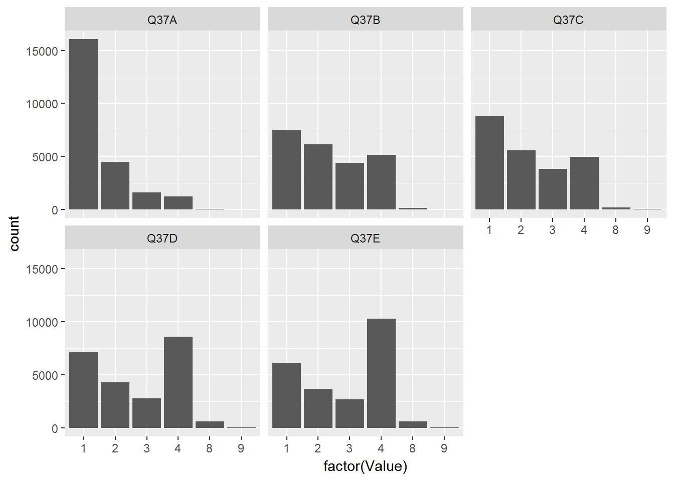
Ok - now we have a bar chart but one that is fairly useless since no one will know what the questions and x-values mean! Let’s add these by appropriate join operations. First add labels to each question:
CountryAttitudesTidy %>%
  left_join(surveyQuestions,by=c("Question"="variable")) %>%
  ggplot(aes(x=factor(Value))) + geom_bar() + facet_wrap(~label)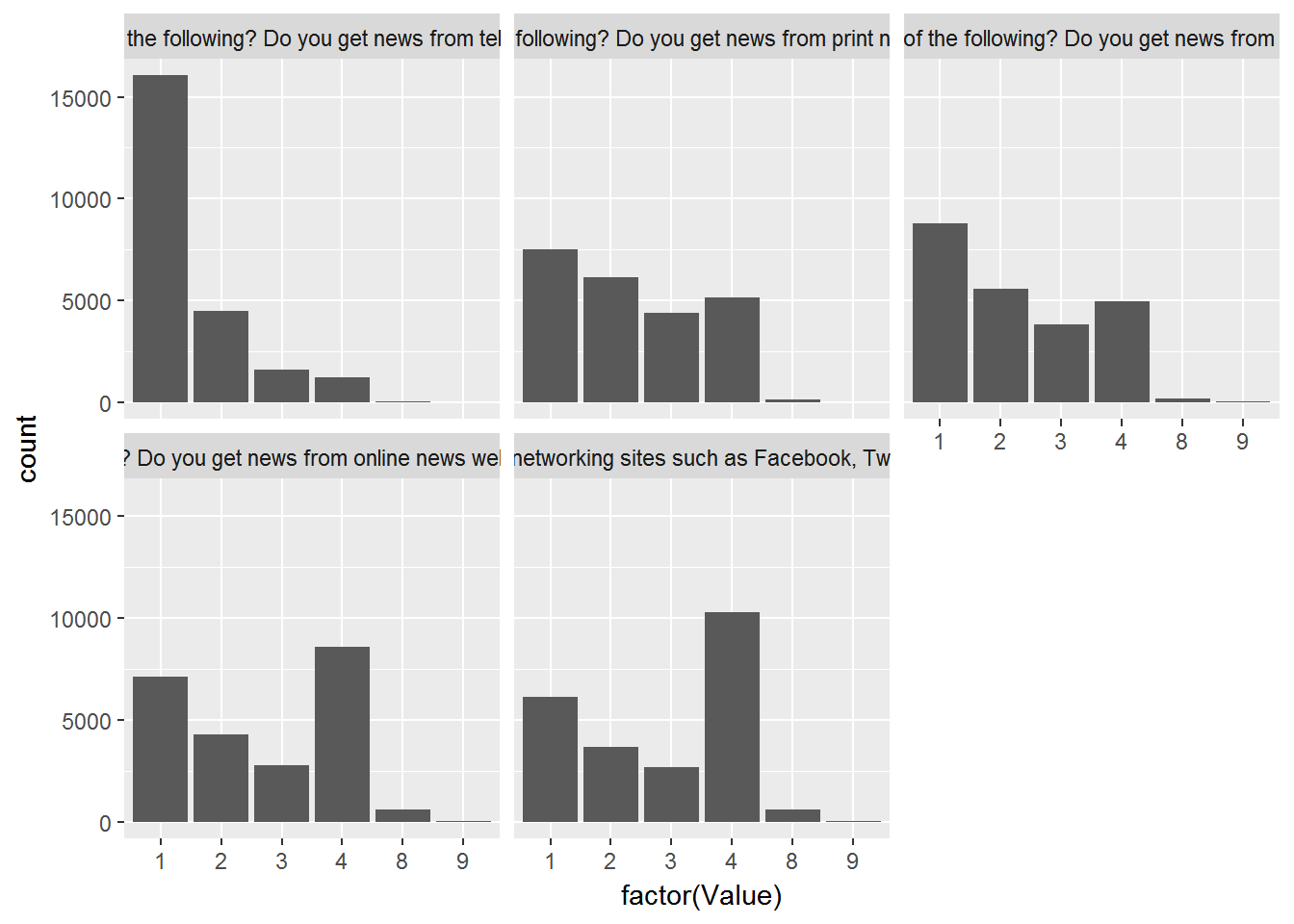
Hmm…that solved the problem but created a new one: The labels are too long so let’s “wrap” in the title bar:
CountryAttitudesTidy %>%
  left_join(surveyQuestions,by=c("Question"="variable")) %>%
  mutate(labelWrap = str_wrap(label,40)) %>%
  ggplot(aes(x=factor(Value))) + geom_bar() + facet_wrap(~labelWrap)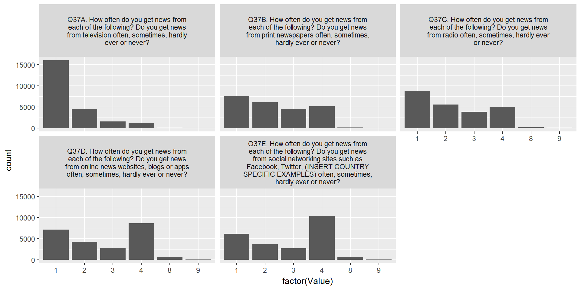
Alright - one problem solved. Now let’s add labels for the x-axis:
CountryAttitudesTidy %>%
  left_join(surveyQuestions,by=c("Question"="variable")) %>%
  mutate(labelWrap = str_wrap(label,40)) %>%
  select(-label) %>%
  left_join(surveyValueLabels,by=c("Question"="question","Value"="value")) %>%
  ggplot(aes(x=label)) + geom_bar() + facet_wrap(~labelWrap) +
  theme(axis.text.x = element_text(angle = 45, hjust = 1))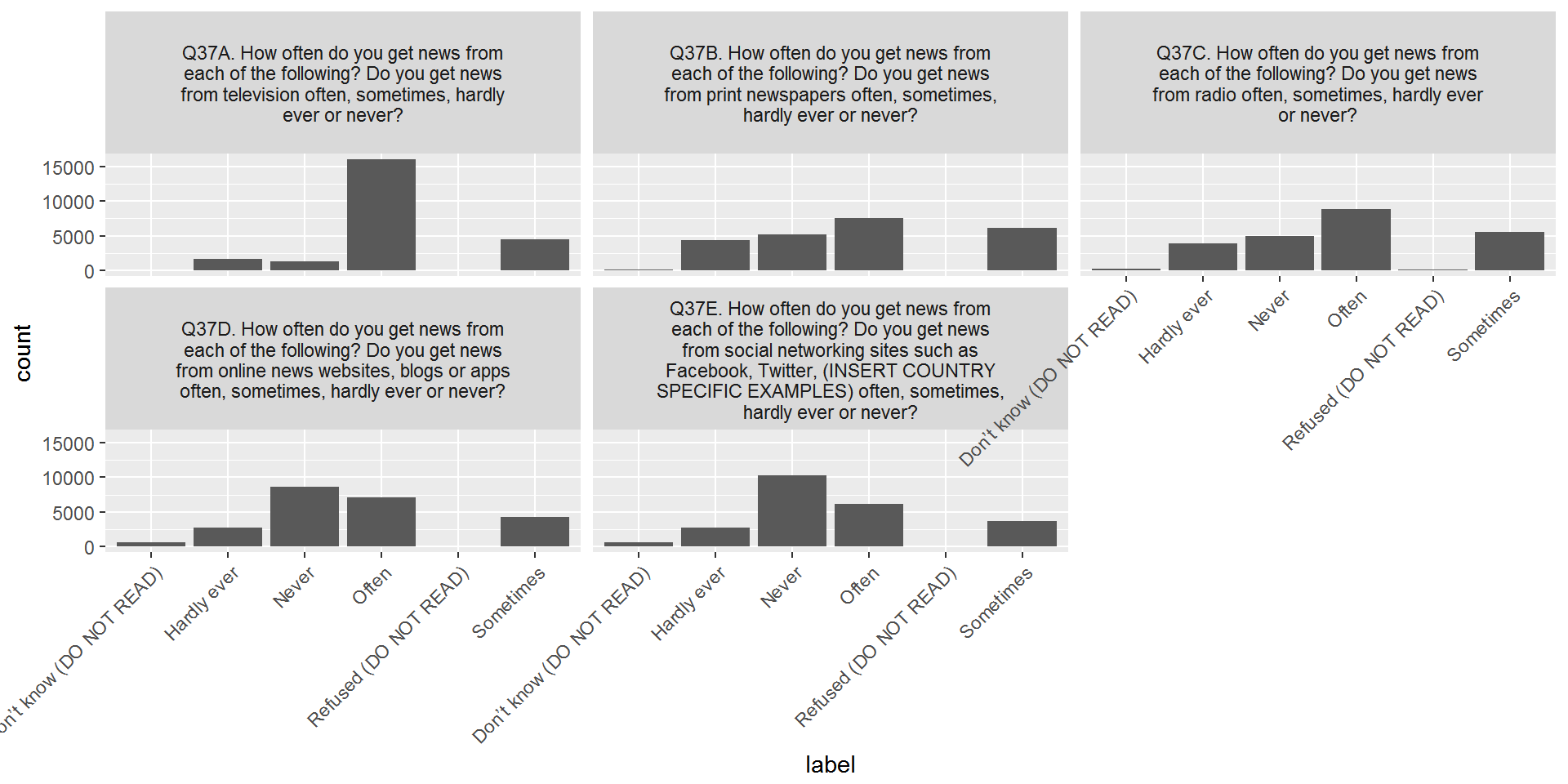
Almost done - let’s remove the answers with very few counts and change the order of the x-axis labels:
CountryAttitudesTidy %>%
  left_join(surveyQuestions,by=c("Question"="variable")) %>%
  mutate(labelWrap = str_wrap(label,40)) %>%
  select(-label) %>%
  left_join(surveyValueLabels,by=c("Question"="question","Value"="value")) %>%
  filter(Value %in% c(1:4)) %>%
  mutate(label = factor(label,levels=c("Often","Sometimes","Hardly ever","Never"))) %>%
  ggplot(aes(x=label)) + geom_bar() + facet_wrap(~labelWrap) + labs(x="Answer")+
  theme(axis.text.x = element_text(angle = 45, hjust = 1))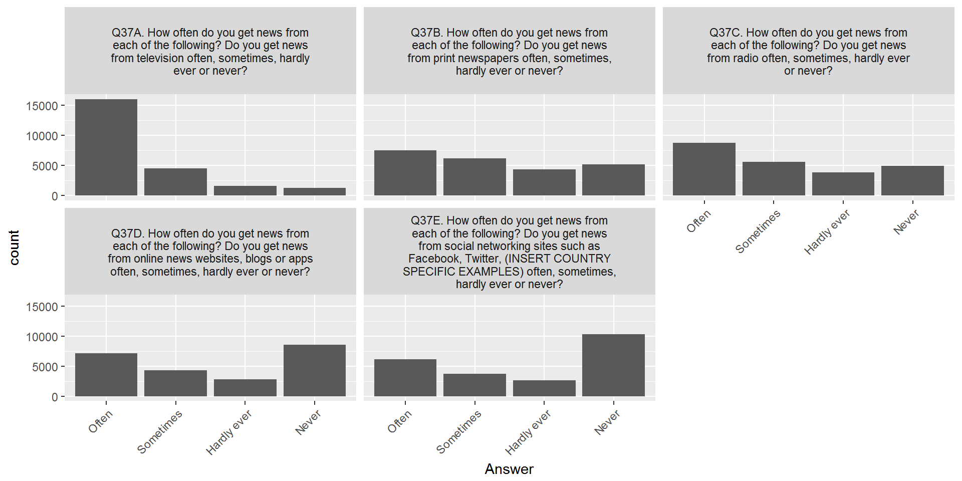
Copyright © 2017 Karsten T. Hansen. All rights reserved.