Collecting Data with an API in R

An increasing popular method for collecting data online is via a Representational State Transfer Application Program Interface. Ok - that’s quite a mouthful and no one really uses the full name but rather REST API or simply API. This refers to a set of protocols that a user can use to query a web service for data. Many organizations make their data available through an API.

There are two ways to collect data with an API in R. The first is to use an R library that comes packaged with functions that call the API. This is by far the easiest since the library developers have already done all the heavy lifting involved in setting up calls to the API. If you can’t find a library that makes calls to the API of interest, then you need to make direct calls to the API yourself. This requires a little bit of more work since you need to look up the documentation of the API to make sure that you are using the correct protocol. Let’s look at some examples.

You can download the code and data for this module as an Rstudio project here.

Using R API-based R packages

There are many R packages that allows a user to collect data via an API. Here we will look at two examples.

Case Study: Google Trends

WWW Google makes many APIs available for public use. One such API is Google Trends. This provides data on query activity of any keyword you can think of. Basically, this data tells you what topics people are interested in getting information on. You can pull this data directly into R via the R package gtrendsR that makes calls to the Google Trends API on your behalf.

First we install the package and then try out a query:

## Install the development version of the gtrendsR package. You only need to run this line once.
devtools::install_github("PMassicotte/gtrendsR")  # only run once

## load library 
library(gtrendsR)

## get web query activity for keyword = "lead" in for queries originating in states of California, Texas, 
## New York and Michigan
res <- gtrends(c("lead poisoning"),geo=c("US-CA","US-TX","US-NY","US-MI"))
plot(res)

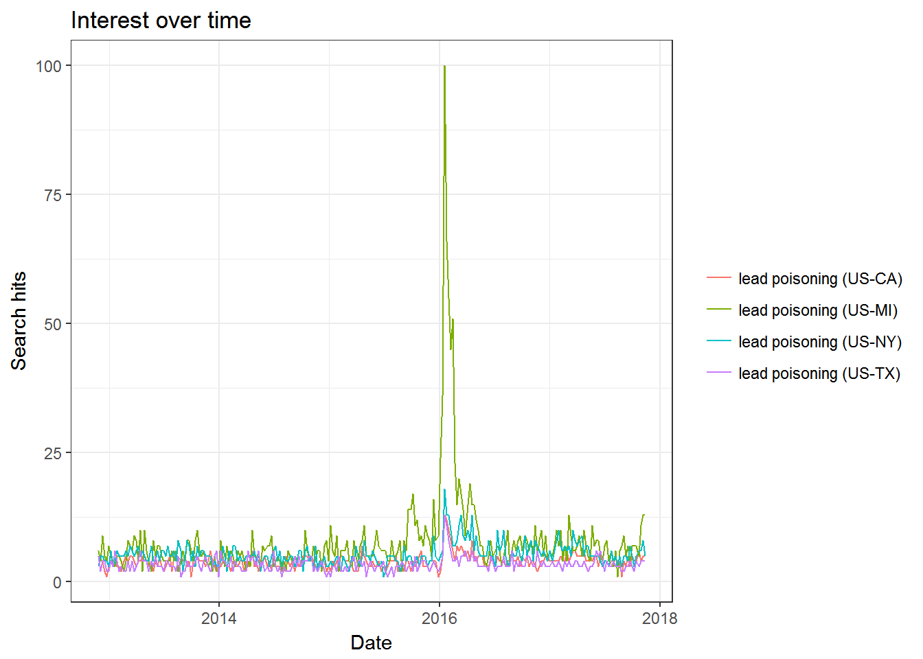
This chart gives us a timeline of daily hits on the keyword “lead poisoning” for four different states. The data has been scaled in the following way: First the “hit rate”" for a given day and geography is calculated. This is the number of searches on the focal keyword divided by all searches on that day (for that geography). The highest hit rate in the data is then normalized to 100 and everything is rescaled relative to that. In the current example we see that the bar far highest hit rate happened in the state of Michigan in early 2016. This makes sense in that a federal state of emergency due to lean in the the drinking water was declared in the town of Flint, Michigan in January 2016. Even before this happened it seems that Michigan had a higher hit rate on this keyword.

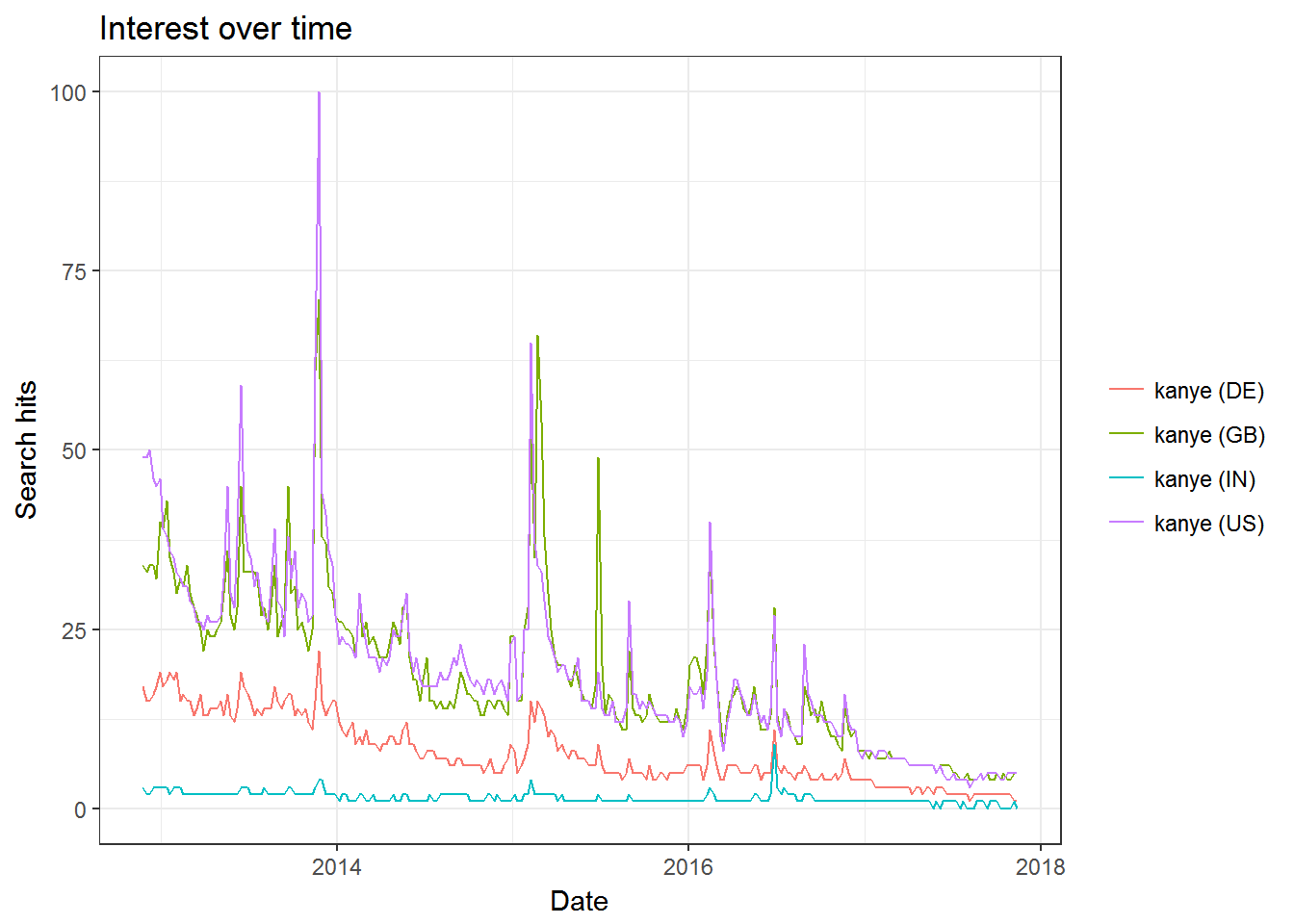
The default source for keyword search is Google web searches. You can change this to other Google products. Here is a visualization of the general decline of Kanye West’s career - as exemplified by popularity on YouTube searches in four countries:

## get Youtube query activity for keyword = "kanye" in USA, Great Britain, Germany, India
res <- gtrends(c("kanye"),geo=c("US","GB","DE","IN"), gprop = "youtube")
plot(res)

The object returned by the gtrends function contain other information than just the timeline. You can also look at search by city within each of the geographies and search hits on related queries:

library(tidyverse)
## get Google Images query activity for keyword = "chris hemsworth" in California and Texas
res <- gtrends(c("chris hemsworth"),geo=c("US-CA","US-TX"), gprop = "images", time = "all")

## plot query activity by city
res$interest_by_city %>%
  mutate(location=factor(location,levels=rev(as.character(location)))) %>%
  ggplot(aes(x=location,y=hits,fill=geo)) + geom_bar(stat='identity') + 
  coord_flip() + 
  facet_wrap(~geo,scales='free') + 
  theme(legend.position = "none")

## plot most popular related queries in California
res$related_queries %>%
  filter(related_queries=="top", geo=="US-CA") %>%
  mutate(value=factor(value,levels=rev(as.character(value))),
         subject=as.numeric(subject)) %>%
  ggplot(aes(x=value,y=subject)) + 
  geom_bar(stat='identity') + 
  coord_flip()

Case Study: Collecting Twitter Data in R

Twitter has an API from which data on tweet activity can be obtained. The R package rtweet contain functions that query this API. In order to use this API you need to have an API key and secret. You can get this for free by registering as a developer. See here for the details.

Let’s use this API to collect tweets mentioning the new iPhone X:

library(rtweet)
appname <- "your app name"
key <- "your API key"
secret <- "your API secret"

twitter_token <- create_token(
  app = appname,
  consumer_key = key,
  consumer_secret = secret)

## collect and save most recent 10,000 English language tweets mentioning "iphonex"
iPhoneX <- search_tweets("iphonex", type = "recent", n = 10000, lang = "en")
saveRDS(iPhoneX,file='data/iphone_tweets.rds')

Here are the fields collected by this API:

names(iPhoneX)

##  [1] "screen_name"                    "user_id"                       
##  [3] "created_at"                     "status_id"                     
##  [5] "text"                           "retweet_count"                 
##  [7] "favorite_count"                 "is_quote_status"               
##  [9] "quote_status_id"                "is_retweet"                    
## [11] "retweet_status_id"              "in_reply_to_status_status_id"  
## [13] "in_reply_to_status_user_id"     "in_reply_to_status_screen_name"
## [15] "lang"                           "source"                        
## [17] "media_id"                       "media_url"                     
## [19] "media_url_expanded"             "urls"                          
## [21] "urls_display"                   "urls_expanded"                 
## [23] "mentions_screen_name"           "mentions_user_id"              
## [25] "symbols"                        "hashtags"                      
## [27] "coordinates"                    "place_id"                      
## [29] "place_type"                     "place_name"                    
## [31] "place_full_name"                "country_code"                  
## [33] "country"                        "bounding_box_coordinates"      
## [35] "bounding_box_type"

The first two tweets in the data are

iPhoneX$text[1:2]

## [1] "RT @gankstars: <f0><U+009F><U+008E><U+0089> #iPhoneX #Giveaway <f0><U+009F><U+008E><U+0089>\n-Tag Your Friends\n-Turn Notifications On\n-RT, Like &amp; Follow @Gankstars\nClick Here: https://t.co/wZnb5<U+0085>"
## [2] "Greenpeace: Why buy the new Apple<U+0092>s #iPhoneX if you can fix your old one?\nhttps://t.co/NQqlHWkor1 https://t.co/mr3vcMne3L"

Here are the top 5 platforms from where the tweets originate:

sort(table(iPhoneX$source),decreasing = T)[1:5]

## 
##          Twitter Lite    Twitter for iPhone   Twitter for Android 
##                  2490                  2080                  1670 
##    Twitter Web Client Gleam Competition App 
##                  1321                   504

Here is the location of the users tweeting the first 20 tweets in the data:

iPhoneX.Users <- users_data(iPhoneX)
iPhoneX.Users$location[1:20]

##  [1] "Zimbabwe"                    "Eger, Magyarország"         
##  [3] "India"                       "29.03.17"                   
##  [5] "Quebec"                      "Tehran, IRAN"               
##  [7] "Redondo Beach, CA"           NA                           
##  [9] "United Kingdom"              "South West, England"        
## [11] "Global"                      "København, Danmark"         
## [13] "Jalgaon, India"              "Narnia "                    
## [15] "India"                       NA                           
## [17] "Mumbai, Ahmedabad, Kolkata " "India"                      
## [19] "New York"                    "Arizona, USA"

Case Study: Computer Vision using Google Vision

Both Google and Microsoft have advanced computer vision algorithms available for public use through APIs. Here we will focus on Google’s version (see here for more detail on Google Vision and here for Microsoft’s computer vision API).

Computer Vision allows you to learn about the features of a digital image. You can do all of this through an API in R as packaged in the RoogleVision package. Let’s try it out.

We first load the required libraries and - as always - install them first if you haven’t already.

# install.packages("magick") 
# install.packages("googleAuthR") 
# install.packages("RoogleVision") 
library(magick)               # library for image manipulation
library(googleAuthR)          # library for authorizing Google cloud access
library(RoogleVision)         # library for Google Vision API calls
library(tidyverse)

First we need to authorize access to Google’s cloud computing platform. You need an account to do this (it is free). Go here to sign up. Once you have an account to create a project, enable billing (they will not charge you) and enable the Google Cloud Vision API (Go to “Dashboard” under “APIs & Services” to do this). Then click on “Credentials” under “APIs & Services” amnd finally “Create credentials” to get your client id and client secret. Once you have obtained these you then call the gar_auth function in the googleAuthR library and you are good to go!

options("googleAuthR.client_id" = "Your Client ID")
options("googleAuthR.client_secret" = "Your Client Secret")

options("googleAuthR.scopes.selected" = c("https://www.googleapis.com/auth/cloud-platform"))
googleAuthR::gar_auth()

You can now call the GoogleVision API with an image. We can read an image into R by using the magick library:

the_pic_file <- 'images/luna.jpg'
Kpic <- image_read(the_pic_file) 
print(Kpic)

WWW

Let’s see what Google Vision thinks this is an image of. We use the option “LABEL_DETECTION” to get features of an image:

PicVisionStats = getGoogleVisionResponse(the_pic_file,feature = 'LABEL_DETECTION',numResults = 20)
PicVisionStats

##           mid        description     score
## 1   /m/0bt9lr                dog 0.9696646
## 2    /m/0kpmf          dog breed 0.9229928
## 3    /m/0km3f labrador retriever 0.9158563
## 4    /m/01z5f    dog like mammal 0.9103422
## 5   /m/05mqq3              snout 0.7814822
## 6   /m/020xxc          retriever 0.6562485
## 7  /m/0265rtm     sporting group 0.6044561
## 8  /m/03yddhn            borador 0.5878804
## 9  /m/02xl47d    dog breed group 0.5299466
## 10  /m/01l7qd           whiskers 0.5074827

The numbers are feature scores with higher being more likely (max of 1). In this case the algorithm does remarkably well. Let’s try another image:

the_pic_file <- 'images/bike.jpg'
Kpic <- image_read(the_pic_file) 
print(Kpic)

WWW

Ok - in this case we get:

PicVisionStats = getGoogleVisionResponse(the_pic_file,feature = 'LABEL_DETECTION',numResults = 20)
PicVisionStats

##           mid             description     score
## 1    /m/0199g                 bicycle 0.9707485
## 2   /m/01bqk0           bicycle wheel 0.9614270
## 3   /m/01bqgn           bicycle frame 0.9247220
## 4   /m/0g7v8f          bicycle saddle 0.9149650
## 5   /m/079bkr       mode of transport 0.8749661
## 6    /m/0_mjp           mountain bike 0.8688098
## 7    /m/0h9mv                    tire 0.8196480
## 8   /m/012f08           motor vehicle 0.8194216
## 9    /m/09rgp            road bicycle 0.7834299
## 10 /m/0h8pb3l         automotive tire 0.7818373
## 11   /m/083wq                   wheel 0.7758130
## 12  /m/03p2h9          hybrid bicycle 0.7592102
## 13 /m/0h8mhph            bicycle part 0.7565305
## 14 /m/0h8m1ct       bicycle accessory 0.6912137
## 15  /m/05y5lj        sports equipment 0.6751224
## 16 /m/06w7n5d                bmx bike 0.6736838
## 17  /m/016xt7                   spoke 0.6172439
## 18   /m/07yv9                 vehicle 0.5764406
## 19 /m/047vmg8                     rim 0.5569364
## 20 /m/0h8ly30 automotive wheel system 0.5005869

Again the algorithm does really well in detecting the features of the image.

You can also use the API for human face recognition. Let’s read in an image of a face:

the_pic_file <- 'images/Karsten4.jpg'
Kpic <- image_read(the_pic_file) 
print(Kpic)

WWW

We now call the API with the option “FACE_DETECTION”:

PicVisionStats = getGoogleVisionResponse(the_pic_file,feature = 'FACE_DETECTION')

The returned object contains a number of different features of the face in the image. For example, we can ask where the different elements of the face are located in the image and plot a bounding box around the actual face:

xs1 = KarstenPicVisionStats$fdBoundingPoly$vertices[[1]][1][[1]]
ys1 = KarstenPicVisionStats$fdBoundingPoly$vertices[[1]][2][[1]]

xs2 = KarstenPicVisionStats$landmarks[[1]][[2]][[1]]
ys2 = KarstenPicVisionStats$landmarks[[1]][[2]][[2]]

img <- image_draw(Kpic)
rect(xs1[1],ys1[1],xs1[3],ys1[3],border = "red", lty = "dashed", lwd = 1)
text(xs2,ys2,labels=KarstenPicVisionStats$landmarks[[1]]$type,col="red",cex=0.9)

dev.off()
print(img)

WWW

Here we see that the API with great success has identified the different elements of the face. The API returns other features too:

glimpse(PicVisionStats)

## Observations: 1
## Variables: 1
## $ error <fctr> No features detected!

Here we see that the algorithm considers it likely that the face in the image exhibits surprise (but not joy, sorrow or anger). It also considers it likely that the person in the image has headwear (which is clearly wrong in this case).

How about this one?

WWW

the_pic_file <- 'images/Karsten1.jpg'
PicVisionStats = getGoogleVisionResponse(the_pic_file,feature = 'FACE_DETECTION')
glimpse(PicVisionStats)

## Observations: 1
## Variables: 15
## $ boundingPoly           <data.frame> 58, 813, 813, 58, 162, 162, 1040...
## $ fdBoundingPoly         <data.frame> 200, 719, 719, 200, 443, 443, 96...
## $ landmarks              <list> <c("LEFT_EYE", "RIGHT_EYE", "LEFT_OF_L...
## $ rollAngle              <dbl> 3.507084
## $ panAngle               <dbl> 2.004963
## $ tiltAngle              <dbl> -11.01594
## $ detectionConfidence    <dbl> 0.9840806
## $ landmarkingConfidence  <dbl> 0.3570419
## $ joyLikelihood          <chr> "VERY_UNLIKELY"
## $ sorrowLikelihood       <chr> "LIKELY"
## $ angerLikelihood        <chr> "VERY_UNLIKELY"
## $ surpriseLikelihood     <chr> "VERY_UNLIKELY"
## $ underExposedLikelihood <chr> "VERY_UNLIKELY"
## $ blurredLikelihood      <chr> "VERY_UNLIKELY"
## $ headwearLikelihood     <chr> "POSSIBLE"

Pretty good! (except for the ceiling light that is still interpreted as head gear).

Querying an API Manually

If you want to query an API for which there is no R package, you need to set up the queries manually. This can be done by use of the GET function in the httr package. The argument to this function will be driven by the protocol of the particular API you are interested in. To find out what this protocol is, you need to look up the API documentation.

Case Study: Collecting Data from The Washington Metropolitan Area Transport Authority

WWW The Washington Metropolitan Area Transport Authority has a nice and well documented API. Let’s use this to collect data on the current positions of all buses on a given bus route. To do this you first have to register on their site. You can do that here. You will then be given an API key you can use for data collection.

There are several APIs available for use. Here we will focus on one returning real time bus positions. In the code below we call the API asking for the current position of all buses on the S4 bus route. To get the correct string argument to the GET function below, just look up the documentation on the bus positions API. The API returns an R list of data that we immediately convert to an R data frame. Finally we plot the results on a nice interactive leaflet map:

library(leaflet)
library(httr)
myApiKey <- "your api key"

## plot current positions of all active busses on route S4
TheRoute <- "S4"
BusGet <- GET(paste0("https://api.wmata.com/Bus.svc/json/jBusPositions?RouteID=",
                     TheRoute,
                     "&api_key=",
                     myApiKey))
BusResult <- content(BusGet)

## convert result to an R data frame
BusResultDF <- do.call(rbind.data.frame,BusResult$BusPositions) 

## plot bus location on an R leaflet map
leaflet(BusResultDF) %>% 
  addTiles() %>%
  addCircles(lng = ~Lon, lat = ~Lat, radius = 200, popup = ~VehicleID)