Linking SQL Databases to R
There are times where you are faced with data of such a magnitude that reading the entire dataset into R - which requires that it fits in your computers memory - becomes problematic. One radical solution to this is: buy more memory! Ok - but what if you don’t want to do that? Is there a way where we can just leave the data in an external file and then pull the relevant sections of it whenever we need it? Yes. The standard here is a SQL database. Technically, “SQL” refers to the language used to make requests to the database but - using the power of R - we actually don’t need to know any SQL syntax to use a SQL database. There are different formats of SQL databases - in the following we will use a sqlite database as an example. This is becoming a very popular database format - in part because it ports easily to mobile platforms.
You can download all the code and data for this module as an Rstudio project here.
SQL Soccer
The file soccer.zip is a zip file containing a sqlite database on over 25,000 soccer matches for 11 European leagues in the period 2008-2016. This database has been assembled by Hugo Mathien - you can read more about the data here. If you want to try out the following code you need to first unzip the zip file (total size is around 311 MB).
You first need to install the RSQLite library (if you haven’t already). Then you need to tell R where the sqlite data is on your computer:
install.packages(RSQLite)    #only do this once
library(tidyverse)

# connect to sqlite database
my_db <- src_sqlite("data/database.sqlite",create = F)
That’s pretty much it - R now has a direct line to the database and you can start making requests.
A SQL database will typically contain multiple “tables”. You can think of these as R data frames. What are the tables in the soccer database?
my_db## src: sqlite 3.8.6 [../data/database.sqlite]
## tbls: Country, League, Match, Player, Player_Stats, sqlite_sequence, TeamOk - we have tables for country, league, match, player and so on. Let’s look at the country and league tables:
country = tbl(my_db,"Country")
league = tbl(my_db,"League")

as.data.frame(country)
## id name
## 1 1 Belgium
## 2 1729 England
## 3 4735 France
## 4 7775 Germany
## 5 10223 Italy
## 6 13240 Netherlands
## 7 15688 Poland
## 8 17608 Portugal
## 9 19660 Scotland
## 10 21484 Spain
## 11 24524 Switzerlandas.data.frame(league)## id country_id name
## 1 1 1 Belgium Jupiler League
## 2 1729 1729 England Premier League
## 3 4735 4735 France Ligue 1
## 4 7775 7775 Germany 1. Bundesliga
## 5 10223 10223 Italy Serie A
## 6 13240 13240 Netherlands Eredivisie
## 7 15688 15688 Poland Ekstraklasa
## 8 17608 17608 Portugal Liga ZON Sagres
## 9 19660 19660 Scotland Premier League
## 10 21484 21484 Spain LIGA BBVA
## 11 24524 24524 Switzerland Super LeagueSo each country has its own league. Let’s do a quick data summary: calculate the average number of goals per league (i.e., country) and plot the averages in a chart:
# calculate average number of goals per country league
goals.match.country = tbl(my_db,"Match") %>%
  group_by(country_id) %>%
  summarise(avg.goal=mean(home_team_goal+away_team_goal)) %>%
  left_join(country,by=c("country_id"="id")) %>%
  arrange(desc(avg.goal))

# plot results
library(forcats)
as.data.frame(goals.match.country) %>%
  ggplot(aes(x=fct_reorder(name,avg.goal),y=avg.goal)) + geom_point() +
ylab('Average Number of Goals per Match') + xlab('National League') + coord_flip() 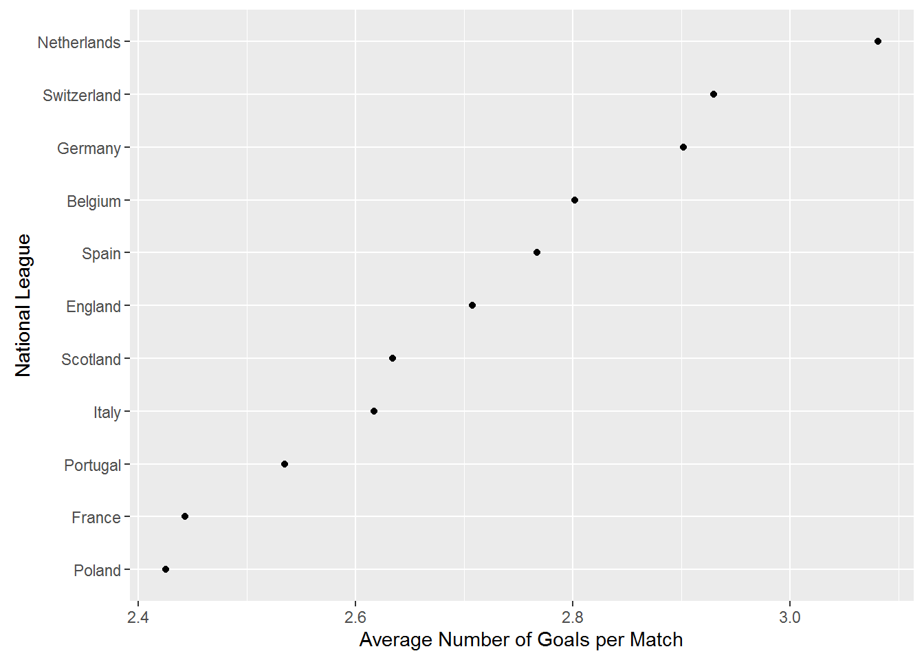
Copyright © 2016 Karsten T. Hansen. All rights reserved.